What is the Analytic Hierarchy Process (AHP)?

The Analytic Hierarchy Process (AHP), sometimes also referred to as the Analytical Hierarchy Process, is a decision-making method used by individuals and organizations to rank alternatives they are considering based on pairwise comparisons (Saaty 1977, 1980).
This article presents a step-by-step guide to implementing the Analytic Hierarchy Process, including a worked example to demystify the calculations. After a discussion of AHP’s strengths and weaknesses, the article concludes by contrasting AHP with a well-known alternative method also based on pairwise comparisons
What is the Analytic Hierarchy Process (AHP)?
Developed by Thomas Saaty in the 1970s at the Wharton School of the University of Pennsylvania, the Analytic Hierarchy Process (AHP) is a multi-criteria decision analysis (MCDA) method that begins by breaking down decisions into a hierarchical structure of a decision-making goal, criteria and alternatives.
The criteria are then weighted and the alternatives scored relative to each other based on the decision-maker performing a series of pairwise comparisons. This weighting and scoring process leads to the generation of a total score for each alternative, by which they are ranked.
AHP is widely used for decision-making in many fields, including business, government, engineering, health care and education.

Analytic Hierarchy Process (AHP): A five-step overview
AHP involves the five steps summarized below. The steps are explained in more detail and illustrated with a worked example in the next section.
1. Structure the hierarchy
The first step of AHP is to organize the main components of your decision-making problem into a hierarchy comprising at least three levels:
-
the over-arching decision-making goal you are trying to achieve, such as:
- “I want to rank smartphones so I can choose one to buy.”
- “Our company wants to short-list applicants for a job.”
- “Our country wants to prioritize responses to climate change.”
- your criteria, and, potentially, any sub-criteria, you are basing the decision on
- the alternatives you are considering
2. Pairwise compare your criteria
The second step of AHP is to assess the relative importance of your criteria (and, potentially, sub-criteria).
This assessment is undertaken via a series of pairwise comparisons of the criteria by answering questions like this: “How much more important is criterion A than criterion B?”
And then for criterion A versus C, and A versus D, B versus C, etc, until you have pairwise compared all your criteria.
Fundamental to AHP is the requirement that you answer the pairwise comparison questions by choosing your answer from a nine-point scale representing the intensity of your preferences, ranging from “equally important” (ratio = 1) to “extreme importance” (ratio = 9).
Alternatively, if you think a criterion is less important than another, this equates to using reciprocals of the nine-point scale, i.e. ratios from 1 (“equally unimportant”) to 1/9 (“extreme unimportance”).
3. Calculate criterion weights
The weights on your criteria, representing their relative importance to you, are derived from the preference ratios elicited at the previous step via some intricate calculations, as illustrated in the worked example later below. These calculations are usually performed using Excel or specialized software.
4. Evaluate alternatives
Having determined the weights on your criteria, the fourth step of AHP is to rate the alternatives you are considering on the criteria.
This evaluation is performed in a similar fashion to how you assessed the relative importance of your criteria, but this time involving a series of pairwise comparisons of the alternatives based on questions like this: “With respect to criterion A, how much more do you prefer alternative X to alternative Y?”
These pairwise comparisons are performed for every pair of alternatives on every criterion.
As for the criteria, you need to answer these questions by choosing from a nine-point scale representing the intensity of your preferences, ranging from “equally preferred” (ratio = 1) to “extremely preferred” (ratio = 9). If you think an alternative is less preferred than another on a criterion, use reciprocals, i.e. from 1 (“equally unpreferred”) to 1/9 (“extremely unpreferred”).
5. Combine weights and scores to rank alternatives
AHP’s final step involves combining the criterion weights from step 3 with the alternatives’ scores from step 5 by multiplying and summing them to get a total score for each alternative, by which they can be ranked.
Thus, like most methods for multi-criteria decision analysis (MCDA), AHP is based on weighted-sum models, also known in the academic literature as additive “multi-criteria value models” or “multi-attribute value models”.
Analytic Hierarchy Process example
AHP’s five steps summarized above are explained in more detail and illustrated here with a worked example accompanied by a workbook you can download if you would like to follow along.
1. Structure the hierarchy
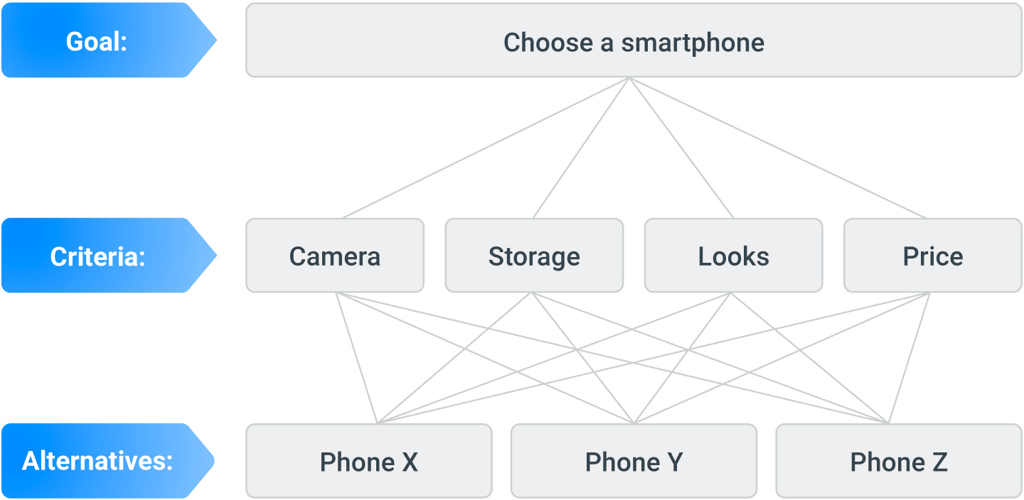
The first step of AHP is to organize the components of your decision-making problem into a hierarchy, where the hierarchy’s first level amounts to being clear about your over-arching decision-making goal – e.g. “I want to rank smartphones so I can choose one to buy”.
The second level involves identifying the criteria that matter to you when evaluating the alternatives you are considering for achieving your goal, and the third level is those alternatives – e.g. criteria for choosing a smartphone might include “camera”, “storage”, “looks” and “price”, and the alternatives are smartphone models.
It can sometimes be useful to further decompose your criteria into various sub-criteria which would form another level of the hierarchy – e.g. “camera” could be broken down into “for taking photos” and “for taking videos”.
The simple three-level hierarchical structure outlined above can be represented by a tree diagram like this:
2. Pairwise compare your criteria
The second step of the Analytic Hierarchy Process is for you to assess the relative importance of your criteria. This assessment is performed via a series of pairwise comparisons, often in the form of a pairwise comparison chart, also known as a pairwise comparison table or matrix.
To get started, create a pairwise comparison chart (matrix) by entering your criteria both down the left-hand side and across the top:
| Camera | Storage | Looks | Price | |
|---|---|---|---|---|
| Camera | ||||
| Storage | ||||
| Looks | ||||
| Price |
Next, go through each cell in the chart, one-by-one, and ask yourself: “How much more important is the criterion in the row than the criterion in the column?” – e.g. “How much more important is “camera” than “storage”?
With respect to your answers, fundamental to AHP are the following ratio scale values and corresponding verbal descriptions that are intended to capture the intensity of your preferences – e.g. where “3” means the row criterion is “3-times as important” as the column criterion, corresponding to “moderately more important”.
1: Equally important
2: Equally to moderately more important
3: Moderately more important
4: Moderately to strongly more important
5: Strongly more important
6: Strongly to very strongly more important
7: Very strongly more important
8: Very strongly to extremely more important
9: Extremely more important
Alternatively, if you think the row criterion is less important than the column criterion, use reciprocals of the numbers above to quantify the relative importance: 1, 1/2, 1/3, 1/4, 1/5, 1/6, 1/7, 1/8 or 1/9 – e.g. where “1/9” means the row criterion is “1/9th as important” as the column criterion, corresponding to “extremely unimportant”.
Thus, AHP requires you to pairwise rate the criteria on, in effect, a 17-point scale, resulting in the pairwise comparison table being filled in like this (where the 1s down the diagonal are criterion self-comparisons, such as “camera” vs “camera”, and are, in effect, filled in by default):
| Camera | Storage | Looks | Price | |
|---|---|---|---|---|
| Camera | 1 | 1/5 | 3 | 4 |
| Storage | 5 | 1 | 9 | 7 |
| Looks | 1/3 | 1/9 | 1 | 2 |
| Price | 1/4 | 1/7 | 1/2 | 1 |
Notice that matching entries in the chart are reciprocal: e.g. if you say “camera” is 4-times as important as “price”, then “price” should be 1/4 as important as “camera”.
3. Calculate criterion weights
The weights on the criteria, representing their relative importance, are derived from your preference ratios in the pairwise comparison chart (matrix) via some intricate calculations usually performed using Excel or specialized software.
After summarizing the steps for performing the calculations, we’ll take you through each step in turn to give you confidence by demystifying them.
The calculations, which are based on an eigenvalue and power method, involve the following five steps. Other methods are available and produce similar results; e.g. see the comparative study by Ishizaka and Lusti (2006).
-
Square the pairwise comparison matrix.
-
Sum each row of the squared matrix to get a “row total” for each row.
-
Sum the “row totals” and then divide each “row total” by the sum. The resulting “priority vector” corresponds to the criterion weights (summing to 1).
-
Using the resulting matrix from step 1, repeat steps 1-3.
-
Repeat step 4 until there are no further significant changes to the priority vector (weights), e.g. to three or four decimal places of accuracy.
If you have any sub-criteria in your decision hierarchy, these steps are performed with your sub-criteria to find their weights too.
Let’s run through an example!
Here is the earlier pairwise comparison table with the fractions now expressed in decimal form, from which the criterion weights will be derived by following the five steps:
| Camera | Storage | Looks | Price | |
|---|---|---|---|---|
| Camera | 1 | 0.2 | 3 | 4 |
| Storage | 5 | 1 | 9 | 7 |
| Looks | 1 | 2 | ||
| Price | 0.25 | 0.1429… | 0.5 | 1 |
Step 1 is to square this matrix – i.e. multiply the matrix by itself – which involves calculating its “dot products”.
Start by multiplying each number in the “camera” row by the corresponding number in the “camera” column and sum the products: (1 × 1) + (0.2 × 5) + (3 × 0.33̇̇) + (4 × 0.25) = 4. This first “dot product” appears in the top-left cell of the squared matrix below. The other 15 dot products are calculated analogously.
Thus, next multiply each number in the “camera” row as above but this time by the corresponding number in the “storage” column, and again sum the products (= 1.305); and then multiply the “camera” row by the “looks” column and sum the products (9.800), and, finally, multiply the “camera” row by the “price” column and sum the products (15.400). Then, move down to the “storage” row and repeat the multiplications/summations outlined above for each of the columns; and then for the “looks” row; and, finally, the “price” row.
Thus, after squaring the matrix above, we have:
| Camera | Storage | Looks | Price | |
|---|---|---|---|---|
| Camera | 4.000 | 1.305 | 9.800 | 15.400 |
| Storage | 14.750 | 4.000 | 36.500 | 52.000 |
| Looks | 1.722 | 0.575 | 4.000 | 6.111 |
| Price | 1.381 | 0.391 | 3.036 | 4.000 |
Step 2 is much easier, just requiring us to sum each row of the squared matrix to get a “row total” for each row:
| Camera | Storage | Looks | Price | Row total | |
|---|---|---|---|---|---|
| Camera | 4.000 | 1.305 | 9.800 | 15.400 | 30.505 |
| Storage | 14.750 | 4.000 | 36.500 | 52.000 | 107.250 |
| Looks | 1.722 | 0.575 | 4.000 | 6.111 | 12.408 |
| Price | 1.381 | 0.391 | 3.036 | 4.000 | 8.808 |
Step 3 is to sum the “row totals and then divide each “row total” by sum. The resulting “priority vector” (final column) corresponds to the criterion weights (summing to 1).
| Camera | Storage | Looks | Price | Row total | Weight | |
|---|---|---|---|---|---|---|
| Camera | 4.000 | 1.305 | 9.800 | 15.400 | 30.505 | 0.192 |
| Storage | 14.750 | 4.000 | 36.500 | 52.000 | 107.250 | 0.675 |
| Looks | 1.722 | 0.575 | 4.000 | 6.111 | 12.408 | 0.078 |
| Price | 1.381 | 0.391 | 3.036 | 4.000 | 8.808 | 0.055 |
| Sum: | 158.971 | 1.000 | ||||
Step 4 is to square the squared pairwise comparison matrix above, and repeat the earlier steps 1-3, resulting in this table and, most importantly, a slightly different set of weights:
| Camera | Storage | Looks | Price | Row total | Weight | |
|---|---|---|---|---|---|---|
| Camera | 73.390 | 22.095 | 172.774 | 250.937 | 519.195 | 0.193 |
| Storage | 252.671 | 76.564 | 594.407 | 866.206 | 1789.848 | 0.667 |
| Looks | 30.692 | 9.235 | 72.402 | 105.290 | 217.620 | 0.081 |
| Price | 22.047 | 6.676 | 52.100 | 76.164 | 156.988 | 0.058 |
| Sum: | 2683.651 | 1.000 | ||||
Step 5 is to repeat step 4 (i.e. again, square the squared, squared pairwise comparison matrix) until there are no further significant changes to the priority vector (weights), e.g. to three or four decimal places of accuracy. In our example, this constancy (convergence) of the final weights is achieved after just one repeat, as above.
Thus, the most important criterion is “storage” (weight = 0.667), followed by “camera” (0.193) and then “looks” (0.081) and – of least importance – “price” (0.058).
Consistency of pairwise comparisons
The consistency of your pairwise comparisons, as summarized in the pairwise comparison chart, can be considered with respect to how well your comparisons satisfy the logical property of transitivity: e.g. if you say “camera” is 2-times as important as “storage”, and “storage” is 3-times as important as “looks”, then – by transitivity – “camera” should be 6-times as important as “looks”.
As well as transitivity, consistency also requires, as discussed earlier, that matching entries in the chart are reciprocal: e.g. if you say “camera” is 4-times as important as “price”, then “price” should be 1/4 as important as “camera”.
Consistency is measured by calculating Saaty’s “consistency ratio” (Saaty 1977, 1980); however, explaining its calculation is outside the scope of this article. A review of consistency measures for AHP is available from Pant et al (2022).
In general terms, and returned to later in the article, the more consistent you are, the higher the “quality” of your judgments in terms of their validity and reliability, and accordingly the more accurate are the weights derived from them.
From a practical perspective, the more consistent your pairwise comparisons, the faster your weights converge at step 5 of the calculations above.
4. Evaluate alternatives
Evaluating the alternatives on the criteria is like assessing the relative importance of your criteria at the previous step. This assessment is also done via a series of pairwise comparisons, again in the form of a pairwise comparison chart (matrix) but this time with a chart for each criterion.
As before, enter the alternatives both down the left-hand side and across the top of each pairwise comparison chart, beginning here with the “camera” criterion:
| Phone X | Phone Y | Phone Z | |
|---|---|---|---|
| Phone X | |||
| Phone Y | |||
| Phone Z |
Next, go through each cell in the chart, one-by-one, and ask yourself: “With respect to this particular criterion, how much more do you prefer the alternative in the row to the alternative in the column?” – e.g. “With respect to their cameras, how much more do you prefer Phone X to Phone Y?
Ask analogous questions for every pair of alternatives on every criterion.
As at step 3, answers to these pairwise comparison questions are chosen from a nine-point ratio scale:
1: Equally preferred
2: Equally to moderately preferred
3: Moderately preferred
4: Moderately to strongly preferred
5: Strongly preferred
6: Strongly to very strongly preferred
7: Very strongly preferred
8: Very strongly to extremely preferred
9: Extremely preferred
If you think the row alternative is less preferred than the column alternative, use reciprocals of the nine-point scale, i.e. from 1 (“equally unpreferred”) to 1/9 (“extremely unpreferred”).
Thus, AHP requires you to pairwise rate the alternatives on a 17-point ratio scale for each criterion, where, again, matching entries in the chart need to be consistent; e.g. if you say Phone X is 6-times more preferred than Phone Z, then Z should be 1/6 as preferred as X:
| Phone X | Phone Y | Phone Z | |
|---|---|---|---|
| Phone X | 1 | 2 | 6 |
| Phone Y | 1/2 | 1 | 3 |
| Phone Z | 1/6 | 1/3 | 1 |
Because there are four criteria for this example, we also need to create a pairwise comparison matrix of the alternatives for the other three criteria (notice, the ratios are all reciprocal, as well as being transitive):
| Phone X | Phone Y | Phone Z | |
|---|---|---|---|
| Phone X | 1 | 1/4 | 1/8 |
| Phone Y | 4 | 1 | 1/2 |
| Phone Z | 8 | 2 | 1 |
| Phone X | Phone Y | Phone Z | |
|---|---|---|---|
| Phone X | 1 | 3 | 9 |
| Phone Y | 1/3 | 1 | 3 |
| Phone Z | 1/9 | 1/3 | 1 |
| Phone X | Phone Y | Phone Z | |
|---|---|---|---|
| Phone X | 1 | 5 | 5 |
| Phone Y | 1/5 | 1 | 1 |
| Phone Z | 1/5 | 1 | 1 |
Finally, in the same way as you did for the criterion weights earlier, calculate the priority vectors for the alternatives – one priority vector per criterion – to obtain scores for each alternative for each criterion by performing these five steps:
-
Square the pairwise comparison matrix.
-
Sum each row of the squared matrix to get a “row total” for each row.
-
Sum the “row totals” and then divide each “row total” by the sum. The resulting “priority vector” corresponds to the alternatives’ scores (summing to 1).
-
Using the resulting matrix from step 1, repeat steps 1-3.
-
Repeat step 4 until there are no further significant changes to the priority vector (scores), e.g. to three or four decimal places of accuracy.
Because the pairwise comparison matrixes above are consistent – both reciprocal and transitive (discussed earlier) – there is no need to perform steps 4 and 5 as the scores will not change, i.e. steps 1-3 are sufficient for consistent matrixes.
The results for each criterion are summarized in the four tables below. In each table, columns 2-4 comprise the squared pairwise comparison matrix (step 1), culminating in the “priority vector” (step 3) in the final column, corresponding to the alternatives’ scores on each criterion.
You might like to check your understanding by downloading our free Excel workbook and having a go at reproducing the four tables yourself (start with decimalized versions of the pairwise comparison charts above).
| Phone X | Phone Y | Phone Z | Row total | Score | |
|---|---|---|---|---|---|
| Phone X | 3.000 | 6.000 | 18.000 | 27.000 | 0.600 |
| Phone Y | 1.500 | 3.000 | 9.000 | 13.500 | 0.300 |
| Phone Z | 0.500 | 1.000 | 3.000 | 4.500 | 0.100 |
| Sum: | 45.000 | 1.000 | |||
| Phone X | Phone Y | Phone Z | Row total | Score | |
|---|---|---|---|---|---|
| Phone X | 3.000 | 0.750 | 0.375 | 4.125 | 0.077 |
| Phone Y | 12.000 | 3.000 | 1.500 | 16.500 | 0.308 |
| Phone Z | 24.000 | 6.000 | 3.000 | 33.000 | 0.615 |
| Sum: | 53.625 | 1.000 | |||
| Phone X | Phone Y | Phone Z | Row total | Score | |
|---|---|---|---|---|---|
| Phone X | 3.000 | 9.000 | 27.000 | 39.000 | 0.692 |
| Phone Y | 1.000 | 3.000 | 9.000 | 13.000 | 0.231 |
| Phone Z | 0.333 | 1.000 | 3.000 | 4.333 | 0.077 |
| Sum: | 56.333 | 1.000 | |||
| Phone X | Phone Y | Phone Z | Row total | Score | |
|---|---|---|---|---|---|
| Phone X | 3.000 | 15.000 | 15.000 | 33.000 | 0.714 |
| Phone Y | 0.600 | 3.000 | 3.000 | 6.600 | 0.143 |
| Phone Z | 0.600 | 3.000 | 3.000 | 6.600 | 0.143 |
| Sum: | 46.200 | 1.000 | |||
As for your criteria, but again outside the scope of this article – and unnecessary for this example – the consistency of your pairwise comparisons of alternatives for each criterion can be evaluated by calculating Saaty’s “consistency ratio”.
5. Combining weights and scores to rank alternatives
The final step of AHP is to combine the criterion weights from step 3 with the alternatives’ scores from step 5.
Weighted-sum model
For each alternative, multiply its score on each criterion by the criterion’s weight and sum the products to get the alternative’s total score, by which the alternatives are ranked.
The total scores for the three phones in our example are calculated from this simple linear equation:
(Wcamera × Scamera) + (Wstorage × Sstorage) + (Wlooks × Slooks) + (Wprice × Sprice),
where the W and S variables are the weights and scores respectively.
Thus, applying the weights and scores from the tables above:
-
Phone X: (0.193 × 0.6) + (0.667 × 0.077) + (0.081 × 0.692) + (0.058 × 0.714) = 0.265
-
Phone Y: (0.193 × 0.3) + (0.667 × 0.308) + (0.081 × 0.231) + (0.058 × 0.143) = 0.290
-
Phone Z: (0.193 × 0.1) + (0.667 × 0.615) + (0.081 × 0.077) + (0.058 × 0.143) = 0.444
Now that we’ve gone through the Analytic Hierarchy Process, we find that Phone Z has the highest total score and so is the best (first), followed by Phone Y in second place and Phone X in third.
Strengths of AHP
AHP is a systematic and logical framework for individuals and organizations to structure decision-making problems and quantify the relative importance of their criteria and the alternatives they are considering to produce a ranking of the alternatives.
As decision-makers work to build the hierarchy of an over-arching decision-making goal, criteria and alternatives, they increase their understanding of the decision-making problem, its context and of how they think and feel about it all.
Finally, as illustrated by the worked example above, AHP is quite straightforward to implement. Albeit the calculations for deriving the criterion weights and alternatives’ scores are intricate, they can be performed using Excel or specialized software.
Weaknesses of AHP
Notwithstanding AHP’s widespread use in many sectors worldwide, many weaknesses have been documented by researchers over the half century since AHP was invented, including Belton & Gear (1983), French (1986) and Belton & Stewart (2002). Munier & Hontoria’s (2021) survey of AHP’s “structural inability for handling complex scenarios” collated criticisms from 101 researchers, grouped under 30 subject headings.
Many of AHP’s weaknesses are technical in nature and outside the scope of this article (if you are interested, consult the citations above). The following four weaknesses, which are widely known, are explained here because, as well as being important, they are easy to understand.
Meaning of AHP’s 1-9 scale
Fundamental to AHP is its pairwise comparison questions and their possible 1-9 ratio scale answers and corresponding verbal descriptions of the intensity of decision-makers’ preferences. The scale and values range from 1 = equally important to 9 = extremely more important, with intermediate levels, such as 3 = moderately more important, 5 = strongly more important, 7 = very strongly more important, etc.
Why these levels of intensity and not others? There is no theoretical foundation for equating the values with their verbal descriptions.
And why is AHP’s maximum value 9 – meaning 9-times as important – instead of another, arbitrary maximum – which could be higher or lower?
Inconsistencies in decision-makers’ preferences
As discussed earlier, the extent of consistency or otherwise – inconsistency – in preferences, as captured by entries in a pairwise comparison chart for criteria and alternatives respectively, has two dimensions:
-
That matching entries in the chart are reciprocal: e.g. if you say “camera” is 4-times as important as “price”, then “price” should be 1/4 as important as “camera”.
-
That entries satisfy transitivity: e.g. if “camera” is 2-times as important as “storage” and “storage” is 3-times as important as “looks”, then “camera” should be 6-times as important as “looks”.
Because matching entries in a pairwise comparison chart are easy to observe, ensuring they are reciprocals is straightforward.
On the other hand, ensuring entries satisfy transitivity is much harder, if not impossible in practice, especially when you are comparing more than three criteria or alternatives, as the number of pairwise comparisons – (n2 − n)/2, where n is the number of criteria/alternatives – increases exponentially.
Therefore, the goal is to ensure the pairwise comparison chart is as close to being consistent as possible – in other words, that it meets some threshold of consistency. As mentioned earlier, “consistency ratios” can be used to evaluate how close, or far away, from being consistent you are, and hence how much confidence you can have in the validity and reliability of your criterion weights and alternatives’ scores.
A related issue that is associated with the previous criticism of AHP’s 1-9 scale is illustrated by this simple example: Suppose “camera” is 4-times as important as “storage”, and “storage” is 4-times as important as “looks”; therefore, “camera” should be 16-times as important as “looks”. But the highest point on the ratio scale is 9, i.e. 9-times. Furthermore, in the extreme, if the first two links in this transitivity chain were 9-times as important, then the third link should be 81-times!
AHP does not permit such ratio scale values. AHP’s maximum value is 9 – hence, virtually, guaranteeing that pairwise comparison charts have inconsistencies.
Rank reversals
“Rank reversal” is the phenomenon whereby when a new alternative is introduced to an AHP application, despite this new alternative not affecting any of the original alternatives included in the application, it leads to a change in the original alternatives’ ranking: a rank reversal! (Belton & Gear 1983). Rank reversal is sometimes referred to as a violation of an important axiom of rational decision-making known as “the independence of irrelevant alternatives”.
Thus, imagine if a fourth phone were added to the smartphone example above and this changed how the original three phones, X, Y and Z, are ranked relative to each other – e.g. suppose Phone Z went from being first to third? Such a rank reversal would undermine most people’s confidence in their results.
Cognitive difficulty of ratio-scale measurements
Most people find answering AHP’s pairwise comparison questions cognitively difficult. Thinking about how strongly you feel about one criterion, or alternative, relative to another and expressing that intensity on a 0-9 scale, even with verbal equivalents, is an unnatural decision-making activity that most people have little experience of in their lives.
In contrast, a more natural decision-making activity is to make choices between alternatives, in the process revealing your preferences. Choosing between alternatives is something we all do dozens if not hundreds of times every day: e.g. “would you like coffee or tea?”, “would you prefer an Android or iOS phone?”, “shall we go to a movie or to see a band?”, etc.
PAPRIKA as an alternative to AHP
A more natural, choice-based process for making decisions that was designed to be as cognitively simple and user-friendly as possible, as well as scientifically valid and reliable, is the PAPRIKA method – an acronym for Potentially All Pairwise RanKings of all possible Alternatives (PAPRIKA) (Hansen & Ombler 2008).
Instead of asking you to rate how much more important one criterion or alternative is than another on a 1-9 scale, PAPRIKA simply asks you to choose between two hypothetical alternatives defined on only two criteria at time and involving a trade-off.
Here is an example of a PAPRIKA pairwise comparison question, as implemented by 1000minds:
Thus, like AHP, PAPRIKA is based on questions involving pairwise comparisons, but much simpler ones involving ordinal instead of ratio-scale measurements of your preferences. Therefore, you can have more confidence in your answers.
Such simple questions are repeated with different pairs of hypothetical alternatives, always involving trade-offs between different combinations of your criteria, two at a time.
As you answer each question, PAPRIKA adapts by fully exploiting the mathematical and logical properties of weighted-sum models, including transitivity (discussed earlier), to select your next question so that you are asked the minimum number required and your answers are always consistent. From your answers, mathematical methods based on linear programming determine your criterion weights, which are used to rank any alternatives you are considering.
Thus, PAPRIKA, implemented by 1000minds, is also based on pairwise comparisons but without AHP’s weaknesses.
Conclusion
The Analytic Hierarchy Process (AHP) is a systematic framework for structuring decision-making problems and using pairwise comparisons to quantify the relative importance of the criteria and alternatives to produce a ranking of alternatives. However, AHP’s weaknesses highlight the usefulness of more natural, choice-based decision-making processes also based on pairwise comparisons like 1000minds’ PAPRIKA method, which is available as an alternative approach.
References
V Belton & T Gear (1983), “On a short-coming in Saaty’s method of analytic hierarchies”, Omega 11, 228-30
V Belton & T Stewart (2002), Multiple Criteria Decision Analysis: An Integrated Approach, Kluwer
P Goodwin & G Wright (1998), Decision Analysis for Management Judgement, John Wiley
P Hansen & F Ombler (2008), “A new method for scoring multi-attribute value models using pairwise rankings of alternatives”, Journal of Multi-Criteria Decision Analysis 15, 87-107
N Munier & E Hontoria (2021), Uses and Limitations of the AHP Method, Springer
S French (1986), Decision Theory: An Introduction to the Mathematics of Rationality, Ellis Horwood
S Pant, A Kumar, M Ram, Y Klochkov & H Sharma (2022), “Consistency indices in Analytic Hierarchy Process: A review”, Mathematics 10, 1206
T Saaty (1977), “A scaling method for priorities in hierarchical structures”, Journal of Mathematical Psychology 15, 234-81
T Saaty (1980), The Analytic Hierarchy Process: Planning, Priority Setting, Resource Allocation”, McGraw-Hill