Multi-Criteria Decision Analysis (MCDA/MCDM)

Introduction
Multi-Criteria Decision Analysis (MCDA), also known as Multi-Criteria Decision-Making (MCDM), is about making decisions when multiple criteria (or objectives) need to be considered together in order to rank or choose between alternatives.
This is a comprehensive overview of MCDA / MCDM in general. With a practical emphasis as well as solid theoretical underpinnings, this is an essential resource for practitioners and academics alike. Whether you are new to the area or already familiar with it, this article is for you!
A similarly comprehensive article on pairwise comparison and pairwise ranking is also available.
A 3-minute introduction to MCDA / MCDM

What is Multi-Criteria Decision Analysis used for?
There are many thousands, if not millions, of possible applications for Multi-Criteria Decision Analysis (MCDA), also known as Multiple Criteria Decision Making and Multi-Criteria Decision-Making (MCDM). Most decisions made by individuals and groups that involve ranking or choosing between alternatives (including people) are amenable to MCDA / MCDM.
Here are some mainstream examples of applications from the worlds of business, nonprofits, government, health, education and personal decision-making:
- Short-listing job applicants
- Selecting projects or investments for funding
- Picking microfinance or aid programs for support
- Prioritizing local or central government spending
- Prioritizing patients for access to health care (e.g. NZ health system success story)
- Ranking researchers or students for research grants or scholarships
- Choosing a new home, car or smartphone, etc
Common to these examples and all MCDA applications in general is that they involve alternatives (including people) being ranked or chosen based on considering multiple criteria together. Some applications also include the allocation of budgets or other scarce resources across alternatives, with the objective of maximizing value for money.
Traditional intuitive decision-making compared to MCDA
Of course, considering multiple criteria when ranking or choosing between alternatives is a natural approach for making decisions that is as old and fundamental as human history (see famous quotes). However, “traditional” intuitive decision-making – how most people make their everyday decisions – typically involves evaluating the criteria and the trade-offs between them in an intuitive or holistic fashion.
In contrast, MCDA / MCDM, a sub-discipline of operations research with foundations in economics, psychology and mathematics, is concerned with formally structuring and solving decision problems. Most MCDA methods, which are increasingly supported by specialized software (e.g. 1000minds), involve the explicit weighting of criteria and the trade-offs between them.
Overall, MCDA is intended to reduce biases from decision-makers relying on their “gut feeling”, and also group decision-making failures (e.g. groupthink), that almost inevitably afflict intuitive approaches. By making the weights and associated trade-offs between the criteria explicit in a structured way, MCDA results in better decision-making.
How does Multi-Criteria Decision Analysis work?
MCDA / MCDM, in essence, involves these four key components:
-
Alternatives (or individuals) to be ranked or chosen from
Any number of alternatives may be included in the MCDM – depending on the application, ranging from a minimum of two (otherwise there wouldn’t be a choice to make) up to 10s, 100s, 1000s or even millions of alternatives.
-
Criteria by which the alternatives are evaluated and compared
For most applications, fewer than a dozen criteria is usually sufficient, with 5-8 fairly typical, which may be quantitative or qualitative in nature.
-
Weights representing the relative importance of the criteria
As explained later in the article, there is a variety of methods available for determining the weights on the criteria, representing their relative importance.
-
Decision-makers and potentially other stakeholders, whose preferences are to be represented
Again, depending on the application, any number of decision-makers and potentially other stakeholders may be involved, ranging from just one (e.g. you!) up to many 1000s of people.
MCDA is about getting these four things right! Do so and you’ll be more likely to make the “right” decision (though, of course, there are no guarantees, as things can change or the unexpected happen).
One-off versus repeated applications
MCDA / MCDM tools can be used for one-off (e.g. ranking applicants applying for a job or prioritizing new business projects) or repeated applications (e.g. prioritizing patients as they present for treatment).
One-off applications involve ranking particular alternatives (or individuals) that are already known to, or under consideration by, the decision-maker. In these applications, the number of alternatives is usually in at most the 10s or 100s – e.g. 250 people applying for a job, or 80 business projects to be prioritized.
In contrast, repeated applications involve ranking alternatives in a pool that is continually changing over time, involving potentially many 1000s of alternatives. For example, in health and education applications, new patients or students (alternatives) may need to be prioritized – e.g. for treatment or scholarships – on an ongoing basis (e.g. hourly or daily), including potentially in “real time”.
The dynamism of repeated applications means that the MCDA process needs to be capable of including potentially all hypothetically possible alternatives (including people, e.g. patients or students) that might ever occur. Accordingly, MCDA outputs are increasingly incorporated into information systems (e.g. as used by New Zealand’s Ministry of Health).
Overview of the MCDA / MCDM process
Most MCDA applications are based, at least implicitly, on the process represented in Figure 1 below reproduced from
As represented in the diagram, the iterative nature of the process, with multiple possible feedbacks and cycles, serves to emphasize that MCDA is intended to function as a tool to help people, individually or in groups, to reach a decision – i.e. their decision (made by humans), not the tool’s decision.
As well as more transparent and consistent decision-making, MCDA can also be used to facilitate the participation of a wide range of stakeholders, systematically taking their preferences into account. MCDA results can also be used to communicate and justify the final decision to stakeholders.

A simple example
As an example, imagine that you are an employer who wants to rank applicants applying for a job vacancy that you have to fill.
In short, there are three fundamental things you need to do to create an MCDA model (a more detailed, six-step process is explained later below):
- Specify relevant criteria for evaluating and comparing the job applicants
- Determine weights for the criteria, representing their relative importance to you
- Rate the applicants on the criteria, resulting in a ranking
In this simple example, identifying the relevant criteria is probably quite straight-forward. Most jobs would include these three criteria (and others too perhaps): qualifications, experience and references.
More challenging is likely to be determining accurate weights for the criteria, reflecting their relative importance, so that when you assess the job applicants on the criteria, they are accurately ranked from “best” to “worst”.
To keep the example as simple as possible, suppose there are just two applicants, Romeo and Juliet. After reading their CVs and interviewing them, suppose you rated them on the three criteria as in Table 1 (where, notice, two ratings are qualitative and one is quantitative).
| Criterion | Applicant rating | |
|---|---|---|
| Romeo | Juliet | |
| Qualifications | poor | good |
| Experience | 4 years | 2 years |
| References | good | good |
Given that Romeo and Juliet are the same with respect to their references (both “good”), whether Romeo is “better” or “worse” than Juliet depends on whether qualifications is more important than experience, or vice versa.
A weighted-sum model
An obvious and common-sense approach for aggregating the performance of each alternative (here, job applicant) across multiple criteria is to create a weighted-sum model. Such models are also known as points systems, and other names are mentioned later below too.
This approach involves weighting the criteria to reflect their relative importance, where the weights sum to 1, and scoring each alternative according to its rating on each criterion, usually in the range 0-100. Each alternative’s performance across the criteria is aggregated via a linear (i.e. additive) equation to produce a total score, also in the range 0-100, with the alternatives ranked by their scores.
An example of criterion weights and scores for ranking job applicants appears in Table 2.
| Criterion | Criterion weight | Level | Criterion score |
|---|---|---|---|
| Qualifications | 0.50 | poor | 0 |
| fair | 20 | ||
| good | 80 | ||
| excellent | 100 | ||
| Experience | 0.32 | ≤ 2 years | 0 |
| 3 years | 50 | ||
| > 3 years | 100 | ||
| References | 0.18 | poor | 0 |
| good | 100 |
Applying this model to Romeo’s and Juliet’s ratings on the three criteria (Table 1) generates their total scores (out of a theoretical maximum of 100 points):
-
Romeo’s total score (for poor, > 3 years, good):
(0.5 x 0) + (0.32 x 100) + (0.18 x 100) = 50points -
Juliet’s total score (good, ≤ 2 years, good):
(0.5 x 80) + (0.32 x 0) + (0.18 x 100) = 58points
Based on their total scores, Juliet is ranked ahead of Romeo for the job.
Notice that the hypothetically best candidate, who would have the highest possible rating on each criterion, would get: (0.5 x 100) + (0.32 x 100) + (0.18 x 100) = 100 points.
It should be obvious that even for this simplest of possible examples the ranking of alternatives depends on the criteria and weights used. Different criteria or weights would have resulted in different total scores and possibly the opposite ranking, or an equal ranking. (The weights above were made up for the sake of this simple illustration.)
The successful implementation of MCDA / MCDM – typically for applications involving more criteria or alternatives than this simple example – depends fundamentally on applying valid and reliable criteria and also weights reflecting decision-makers’ preferences (and potentially other stakeholders’ preferences too, depending on the application). As discussed later below, specialized methods are available for eliciting preferences.
Origins of MCDA
Historically, the first example of a formal approach related to Multi-Criteria Decision-Making was described by Benjamin Franklin in 1772 (
Franklin humbly begins his letter with this sentence (which also serves to reassure us that although as individuals we may have different preferences, we can still use the same decision-making methods):
Dear Sir,
In the affair of so much importance to you, wherein you ask my advice, I cannot, for want of sufficient premises, advise you what to determine, but if you please I will tell you how.
Franklin’s method (his “how”) involves first tabulating the “pros” and “cons” of the alternative being evaluated relative to another alternative (e.g. the status quo), and then successively trading them off – in effect, weighting them – in order to identify the better alternative. Though this simple approach is effective for decisions involving choosing between two alternatives, it does not scale up for more alternatives.
More than 200 years later, more technically sophisticated methods for choosing between more than just two alternatives, and potentially involving multiple decision-makers, were presented by Ralph Keeney and Howard Raiffa in their seminal book, Decisions with Multiple Objectives: Preferences and Value Tradeoffs (
In 1979, Stanley Zionts helped popularize the abbreviation MCDM (for Multiple Criteria Decision-Making) with his article for managers: “MCDM – If not a Roman numeral, then what?” (
Other significant events from MCDA’s / MCDM’s history are discussed in the book by Köksalan, Wallenius & Zionts (2011).
MCDA software
Nowadays, Multi-Criteria Decision Analysis is increasingly supported by specialized software (mostly web-based). Before the advent of the World Wide Web in the 1990s, most MCDA / MCDM software was based on spreadsheets, such as the early example described by
MCDA software frees “the facilitator/analyst and decision-maker from the technical implementation details, allowing them to focus on the fundamental value judgments” (
MCDA software is especially useful for applications involving many alternatives and criteria, and when the methods for determining the weights on the criteria (and scoring the alternatives on the criteria) are technically sophisticated.
Also, software capable of surveying potentially 1000s of people is useful for applications based on eliciting and analyzing the preferences of members of the general population (e.g. nationwide surveys).
MCDA software, ranging from the most basic to the state of the art, is catalogued in these three overviews:
- Wikipedia’s “comparison of decision-making software” – an up-to-date list exclusively focused on MCDM software
-
OR/MS Today’s “Decision Analysis Software Survey” (
Beekman 2020 ) – an up-to-date, vendor-completed survey but with a broader focus on decision analysis (DA) software in general (i.e. MCDA / MCDM is a subset of decision analysis) -
Weistroffer & Li’s (2016) survey of “Multiple Criteria Decision Analysis Software” – an exhaustive review of all commercially and academically available MCDM / MCDA software
If you would like to experience a prominent example of MCDA software, 1000minds (implementing the PAPRIKA method, explained later below), you can create yourself a 1000minds account.
The remainder of the article is devoted to explaining the steps for creating and applying weighted-sum models, beginning with a more detailed discussion of weighted-sum models (as introduced earlier). Some of this material is adapted from parts of
Weighted-sum models
As mentioned earlier, most MCDA / MCDM applications are based on weighted-sum models. Such models are also known in the academic literature as additive multi-attribute value models.
As explained earlier (and see Table 2 again), weighted-sum models involve decision-makers explicitly weighting the criteria for the decision problem being addressed and rating the alternatives on the criteria. Each alternative’s overall performance on the criteria is aggregated via a linear (i.e. additive) equation to produce the alternative’s total score, with the alternatives ranked by their scores.
Points systems
A common and equivalent representation of the linear equations at the heart of weighted-sum models is a schedule of point values (sometimes referred to as preference values) for each criterion. These schedules are also known as points systems, and also as additive, linear, scoring, point-count and points models or systems.
The points-system equivalent of the weighted-sum model in Table 2 appears in Table 3. In the table, the point value for each level on a criterion represents the combined effect of the criterion’s relative importance (weight) and its degree of achievement as reflected by the level.
In other words, consistent with the linear equations described above, a level’s point value can be obtained by multiplying the criterion weight by the criterion score from the equation. This relationship can be easily confirmed by multiplying the weights by the scores in Table 2, as reported in the fourth column below (for illustrative purposes). Likewise, a point value can be decomposed – in the opposite direction – into the criterion’s weight and score.
A points-system representation is sometimes preferred because, arguably, a simple schedule of point values is easier to implement than an equation (a set of weights and scores that need to be multiplied together). Also, in tabular form, a points system takes up less space (e.g. compare Table 2 and Table 3).
| Criterion | Level | Points | Illustrative calculation |
|---|---|---|---|
| Qualifications | poor | 0 | 0.5 x 0 |
| fair | 10 | 0.5 x 20 | |
| good | 40 | 0.5 x 80 | |
| excellent | 50 | 0.5 x 100 | |
| Experience | ≤ 2 years | 0 | 0.32 x 0 |
| 3 years | 16 | 0.32 x 50 | |
| > 3 years | 32 | 0.32 x 100 | |
| References | poor | 0 | 0.18 x 0 |
| good | 18 | 0.18 x 100 |
Applying the points system in Table 3 to Romeo’s and Juliet’s ratings on the three criteria (Table 1) generates their total scores:
- Romeo’s total score (for poor, > 3 years, good):
0 + 32 + 18 = 50points - Juliet’s total score (good, ≤ 2 years, good):
40 + 0 + 18 = 58points
Notice that these total scores are the same as before, thereby confirming the equivalence of Tables 2 and 3. Again, based on their total scores, Juliet is ranked ahead of Romeo for the job.
Notice, again, that the hypothetically best candidate, with the highest possible rating on each criterion, would get: 50 + 32 + 18 = 100 points.
Simplicity and accuracy
In practical terms, a major attraction of weighted-sum models – in either their linear equation (Table 2) or points-system (Table 3) forms – is the simplicity by which each alternative’s performance on each criterion is aggregated to produce the alternative’s total score. (Non-linear functions for aggregating the criteria, including multiplicative functions, are also possible but very rare.)
More importantly, such simple models (sometimes referred to as algorithms or formulas) have been found nearly universally in very many studies to be more accurate than the intuitive or holistic judgments of decision-makers (
According to
surprisingly successful in many applications. We say “surprisingly”, because many judges claim that their mental processes are much more complex than the linear summary equations would suggest – although empirically, the equation does a remarkably good job of “capturing” their judgment habits.
Hastie and Dawes (p. 52) also explained:
The mind is in many essential respects a linear weighting and adding device. In fact, much of what we know about the neural networks in the physical brain suggests that a natural computation for such a “machine” is weighting and adding, exactly the fundamental processes that are well described by linear equations.
Also, according to
[Weighted-sum models / points systems] are, as a rule, more accurate than human predictors. This is not surprising, as it has been known for decades that human cognitive performance is limited with respect to complex multi-variable judgment and prediction tasks (
Meehl 1954 ).
Other approaches to Multi-Criteria Decision Analysis
For completeness, it’s worthwhile mentioning that other MCDA-based approaches not based on aggregative functions for combining alternatives’ performance on criteria (i.e. via weights) are also potentially available. These other approaches are available as alternatives to weighted-sum models, albeit they are unlikely to be more useful.
Performance matrices
The most basic alternative approach is a simple table, sometimes referred to as a performance matrix, for reporting the alternatives’ performance on the criteria. In the table/matrix, each alternative is a row and each criterion is a column.
If one alternative dominates the others on all criteria, or where the trade-offs involved in selecting an alternative are clear and uncontroversial, then decision-makers can use such a table to reach their decision quickly.
However, most decision problems are more complicated than this!
Most MCDA / MCDM applications involve confronting non-trivial trade-offs between criteria. Therefore, merely tabulating alternatives’ performance on the criteria is insufficient for most applications. Nonetheless, such a table may be useful at step 3 in the MCDA process outlined in the next section.
Outranking methods
A MCDA / MCDM approach capable of evaluating trade-offs between criteria, but that is not based on aggregative functions for combining alternatives’ performance on criteria (via weights), is the group of outranking methods.
Methods in this tradition include:
- PROMETHEE (
Vincke & Brans 1985 ) – an acronym for “Preference Ranking Organization METHod for Enrichment of Evaluations” - GAIA (
Brans & Mareschal 1994 ) – for “Geometrical Analysis for Interactive Aid” - ELECTRE family of methods (
Roy 1991 ) – for “ELimination Et Choix Traduisant la REalité” (which translates as “elimination and choice expressing reality”)
In essence, outranking methods involve decision-makers pairwise ranking all the alternatives relative to each other on each criterion in turn and then combining these pairwise-ranking results but not via weights. The objective is to obtain measures of support for judging each alternative to be the top-ranked alternative overall.
Relative to weighted-sum models, outranking methods are rarely used. Their unpopularity is probably mostly due to their complexities and the non-intuitive nature of their inputs and algorithms relative to weighted-sum models.
The steps for creating and applying weighted-sum models, including a survey of methods for determining weights, is explained next.
Steps for performing Multi-Criteria Decision Analysis
The steps for creating and applying weighted-sum models (or points systems), likely to be useful for most applications, are summarized in Table 4 and are discussed in turn next. These steps are consistent with the overall MCDA / MCDM process represented in the diagram near the start of the article.
Given the wide range of possible MCDA applications (as mentioned earlier), the steps, as presented here, are necessarily generic. Equivalent processes for specific applications are available in the literature, such as prioritizing patients for access to health care (
Although the steps are presented in sequence below, they do not necessarily need to be performed in that order.
Also, earlier steps, such as step 1 (structuring the decision problem) and step 2 (specifying criteria), can be revisited during the process as new insights into the particular application emerge and revisions and refinements become desirable.
Though, in principle, the steps can be performed “by hand” (e.g. supported by spreadsheets), many of them, and often entire processes, are supported by MCDM software (as discussed above). Such software is especially useful for applications involving many alternatives and criteria, and when the scoring and weighting (step 4) methods are technically sophisticated.
| Step | Brief description |
|---|---|
| 1. Structuring the decision problem |
Identify objectives, alternatives, decision-makers, any other stakeholders, and the output required. |
| 2. Specifying criteria |
Specify criteria for the decision that are relevant to decision-makers (and, potentially, other stakeholders) and preferentially independent. |
| 3. Measuring alternatives’ performance |
Gather information about the performance of the alternatives on the criteria. |
|
4. Scoring alternatives and weighting the criteria |
Convert the alternatives’ performances on the criteria into scores on the criteria, and determine weights for the criteria. |
| 5. Applying scores and weights to rank alternatives |
Multiply alternatives’ scores on the criteria by the weights and sum to get total scores, by which the alternatives are ranked. |
| 6. Supporting decision-making |
Use the MCDA outputs to support decision-making – i.e. ranking or selecting alternatives (depending on the application). |
1. Structuring the decision problem
The first step of the MCDA / MCDM process involves structuring and framing the decision problem being addressed (and see the first stage in the earlier diagram again).
In particular, it’s important to clarify the over-arching objectives of the decision-making exercise, and to think about the overall outcomes that are desired.
Related issues include:
- Identifying the alternatives under consideration
- Whether the decision is a one-off or repeated application (as discussed earlier)
- The type of output required from the MCDM, e.g. a ranking or a selection
These elements should be validated with stakeholders.
2. Specifying criteria
The criteria specified for the decision should be valid, reliable and relevant to decision-makers and other stakeholders. They should also be preferentially independent, as explained below.
The criteria should be structured to avoid double-counting and minimize overlap between them. For example, having criteria for attractiveness and also beauty when choosing a car would invalidate the weighting methods discussed below and their results.
Depending on the application, the criteria can be identified from: similar decisions, reviews of the literature, facilitated discussions, expert opinions, focus groups and surveys. As in the previous step, stakeholders should be involved in identifying and validating the criteria.
For example, 1000minds offers noise audits whereby participants use their intuition to rank real or imaginary alternatives to inspire a discussion of the criteria (as well as to demonstrate how inconsistent decision-makers are and hence the need for a better approach than relying on intuition).
Preferential independence
Part of the requirement that the criteria are valid and reliable includes that they are preferentially independent. This property is most easily explained using an example: Imagine that you are looking for a car to buy, and your criteria include power source (i.e. electric versus fossil fuels) and type of car (modern, classic or vintage).
If your preference for a car to be powered by electricity rather than fossil fuels does not depend on whether the car is modern, classic or vintage, then these two criteria for choosing a car – power source and type of car – are preferentially independent.
If they are not (i.e. if your criteria are preferentially dependent), then you need to re-specify them in such a way that they are (or don’t use these criteria).
Criteria can be preferentially independent despite being highly correlated: e.g. vintage cars almost always run on petrol instead of electricity, and this correlation between the two criteria, power source and type of car, is fine when it comes to specifying them for choosing between cars.
Similarly, in another example, if you were choosing a phone based on the criteria of weight and screen size, given current technology, very light phones have to have small screens. This correlation between weight and screen size is fine as far as their inclusion as criteria is concerned: independence of criteria in relation to the decision-maker’s preferences is what matters, not independence of criteria in relation to real alternatives – we’re allowed to dream of the perfect phone (or car, etc)!
3. Measuring alternatives’ performance
Data about the alternatives’ performance in terms of each of the criteria can be gathered in a variety of ways, ranging from expert opinions to rapid literature reviews, to full systematic reviews and modeling exercises. These data can be presented in a performance matrix or table (as discussed earlier), if useful.
The sophistication and intensity of the data-gathering activity depend on the availability of relevant evidence, the decision problem, and also other practical factors such as the resources available for the job.
MCDA / MCDM is capable of including both quantitative and qualitative data. It is also capable of combining subjective judgments (in the absence of “harder” data) with more traditional scientific evidence in the same application. For example,1000minds has surveying tools for collecting decision-makers’ ratings of the alternatives on the criteria, and for aggregating results.
4. Scoring alternatives and weighting the criteria
Scoring alternatives and weighting criteria are sometimes considered separate steps. They are treated together here because they are intrinsically linked. They can be performed sequentially, simultaneously or iteratively, depending on the application and methods (or software) used.
Scoring alternatives on the criteria
Scoring the alternatives on the criteria involves converting each alternative’s performance on each criterion into a numerical score. The scores are usually normalized so the worst performance on the criterion gets a score of zero and the highest performance gets 100.
Scores on the criteria can be implemented using a continuous scale (0-100). Or, alternatively, as in the example at the beginning of the article, two or more mutually-exclusive and exhaustive levels (e.g. low, medium, high) can be employed, each with a point value (e.g. medium = 60).
Weighting the criteria
Weighting the criteria involves determining their weights, representing their relative importance to decision-makers. The weights are usually normalized to sum across the criteria to one (100%).
Overall, it’s very important that the alternative scores and criterion weights are as valid and reliable as possible.
Otherwise, if the scores or weights are “wrong” (inaccurate), then the “wrong” decision, as determined by the ranking of the alternatives’ total scores, is almost certain – even if valid and reliable criteria have been specified (step 2) and the alternatives’ performances have been accurately measured (step 3).
A variety of methods for scoring alternatives on the criteria and weighting the criteria are available, as discussed in the next section.
5. Applying scores and weights to rank alternatives
Having scored the alternatives on the criteria and weighted the criteria, it’s easy to calculate their total scores (usually performed automatically by MCDA software).
With reference to the scoring and weighting methods explained below:
- For the direct methods and, in effect, the PAPRIKA (choice-based) method, each alternative’s scores on the criteria are multiplied by the weights, and then the weighted scores are summed across the criteria to get each alternative’s total score (e.g. see Table 2 and Table 3 above).
- For the conjoint analysis (or DCE) method, the regression technique estimates each alternative’s value (or utility) or its probability of being preferred by decision-makers.
6. Supporting decision-making
The final step of the MCDA / MCDM process is to use the results, usually presented in tables like the one above, or charts, to support your decision-making – i.e. depending on your application, for ranking or selecting alternatives.
Where appropriate, the MCDM inputs, process and results can be used to communicate and explain the final decision to stakeholders.
As for any analysis based on uncertain inputs, it’s important to perform sensitivity analysis to check the robustness of your results to plausible variations, e.g. in the alternatives’ performance (step 3) and their scores, or on the criterion levels, or in the criterion weights (step 4).
Overall, decision-makers need to understand the MCDM results, including any significant limitations of the analysis. These results can be used to support decision-makers in reaching and, if need be, defending their decision.
It is important to remember, as emphasized at the beginning of the article, that MCDM is intended as a tool to help people, individually or in groups, to reach a decision – their decision (the humans’ decision), not the tool’s decision.
Also, in some applications, other considerations in addition to the MCDM results may also be relevant for the decision being made.
For example, decisions with budgetary implications, such as investment or project decision-making (e.g. CAPEX or OPEX), involve comparing the benefits of each alternative, as represented by their MCDM total score, relative to their costs. Other factors, such as strategic or legal factors, might also be worthwhile considering.
Value-for-money assessments
The MCDA / MCDM process explained above, resulting in a decision-making tool – a weighted-sum model, or points system, comprising criteria and weights – can be complemented by a framework for making resource-allocation decisions based explicitly on value for money and efficiency, as summarized here.
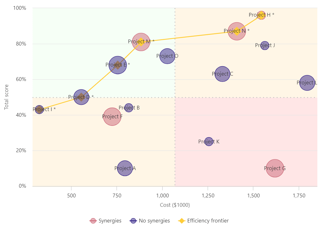
For the simple example of project decision-making subject to a budget, consider the value-for-money (VfM) chart in Figure 2.
The vertical axis of the VfM chart represents each project’s benefit, expressed in terms of a total score, i.e. based on the criteria and weights derived earlier. The horizontal axis displays each project’s estimated cost.
As an illustration, the chart can be used to think about the following questions.
Suppose you had a budget of $8 million.
Which of the 15 projects in the chart – costing more than $16 million, in total – represent high quality spending, e.g. with high benefit-cost ratios?
Which projects would you reject because they represent low quality spending, e.g. that are dominated by the efficient projects?
Thinking about the first question should draw your focus of attention to the chart’s top-left quadrant, i.e. projects with relatively high Benefit (total score) and low Cost.
Possible trade-offs between Cost and Benefit are along the gold line, known as the efficiency or Pareto frontier: higher Cost can be compensated for by higher Benefit.
The size and color of the bubbles in the chart can also be used to represent other potentially important considerations, such as confidence in cost estimates (e.g. high, medium, low), synergies, political support, etc.
In general, applying this value for money framework involves decision-makers considering alternative affordable combinations to arrive at their “optimal portfolio” of projects.
In operations research, this combinatorial optimization problem is an example of the famous “knapsack problem” (Dantzig & Mazur 2007).
Scoring and weighting methods
As noted at step 4 above, a variety of methods for scoring alternatives on the criteria and weighting the criteria are available, often supported by MCDA software (as discussed earlier). For the reasons explained below, these methods can be broadly classified as direct and choice-based methods respectively.
Also, many of the methods explained below involve pairwise comparisons of alternatives or criteria, including pairwise ranking. [A comprehensive overview of pairwise comparisons and pairwise rankings, which, like the present article, is intended as an essential resource for practitioners and academics (including students), is available here.]
Direct methods include:
- Direct rating and points allocation (
Bottomley, Doyle & Green 2000 ) - SMART (
Edwards 1977 ) – an acronym for “Simple MultiAttribute Rating Technique” - SMARTER (
Edwards & Barron 1994 ) – for “Simple MultiAttribute Rating Technique Exploiting Ranks” - Analytic Hierarchy Process (AHP) (
Saaty 1977 ) - Swing weighting
- “Bisection” and “difference” methods (
Winterfeldt & Edwards 1986 )
Choice-based methods include:
- PAPRIKA (
Hansen & Ombler 2008 ) – an acronym for “Potentially All Pairwise RanKings of all possible Alternatives” - Conjoint analysis (or discrete choice experiments, DCE) (
McFadden 1974 ) (Green, Krieger & Wind 2001 )
These eight direct and two choice-based methods are explained in detail in turn below. First, though, the main difference between the two groups of methods – direct and choice-based – are discussed.
Direct versus choice-based methods
Direct methods for scoring alternatives on the criteria involve decision-makers directly expressing how they feel about the relative performance of each alternative on a criterion relative to the other alternatives.
These expressions of a decision-maker’s preferences are usually measured using either an interval scale (e.g. alternatives are rated on a 0-100 scale on a criterion) or a ratio scale (e.g. “alternative A is three times as important as alternative B on a criterion”).
Similarly, direct methods for weighting the criteria involve decision-makers (directly) expressing how they feel about the relative importance of the criteria, again usually represented in terms of either an interval scale (e.g. criteria are rated on a 0-100 scale) or a ratio scale measurement (e.g. “criterion A is three times as important as criterion B”).
Direct methods have the superficial appeal of directly asking the decision-maker about how they feel about the relative importance of the criteria or alternatives, from which scores for the alternatives on each criterion or criterion weights are derived (i.e. directly).
Also, when you read the direct methods’ explanations below, hopefully, you’ll to be struck by their algorithmic and computational simplicity, such that they can be easily implemented “by hand” (e.g. supported by spreadsheets), whereas the choice-based methods require specialized software (which come with other useful features, of course).
Unfortunately, however, these direct methods have the major disadvantage of being based on preference-elicitation tasks that are cognitively difficult for most people, and so the validity and reliability of their results is questionable. For example, expressing how strongly you feel about one criterion (or alternative) relative to another one on a scale ranging from “equally preferred” (ratio = 1) to “extreme importance” (ratio = 9) is not a natural human mental activity that many of us have much experience of.
As an example, suppose you’re an employer looking to hire someone for a job. How easy would you find thinking about a question like this:
On a nine-point scale ranging from “equally preferred” (ratio = 1) to “extreme importance” (ratio = 9), how much more important to you is a person’s qualifications than their experience?
How confident would you be in the accuracy (validity and reliability) of your answer?
In contrast, the choice-based methods explained below involve decision-makers expressing their preferences usually by answering relatively simple questions based on choosing between two or more alternatives defined on some or all of the criteria – an example of such a question appears in Figure 3 below. From these rankings or choices, scores and weights are derived (indirectly) using regression-based techniques or other quantitative methods.
The advantage of these choice-based methods is that choosing between things is a natural type of decision activity experienced by all of us in our daily lives. We make such judgments dozens, if not hundreds, of times every day (e.g. “would you like scrambled or poached eggs for breakfast?”). Therefore, choice-based methods are likely to be more valid and reliable than direct methods, as well as being easier for decision-makers.
In the words of
The advantage of choice-based methods is that choosing, unlike scaling, is a natural human task at which we all have considerable experience, and furthermore it is observable and verifiable.
The eight direct and two choice-based methods are briefly explained in turn below (and more detailed information is available from their references above). Given the advantages of choice-based methods discussed above, you might like to skip to that sub-section.
Direct methods
Each of the following eight methods is explained in terms of scoring alternatives on the criteria, and weighting the criteria.
Direct rating
Scoring alternatives on the criteria
For each criterion, each alternative is rated on a point scale ranging from 0 to 100 in proportion to its performance on the criterion relative to the other alternatives being considered. This rating exercise is typically performed using a visual analogue scale (VAS) or equivalent. (A VAS looks like a household thermometer, either standing up or on its side.)
The alternatives’ scores on the criterion are usually normalized so that the alternative with the lowest (or “worst”) score gets 0 and the one with the highest (“best”) score gets 100.
Weighting the criteria
Each criterion is rated on a point scale ranging from 0 to 100 – e.g. using a VAS (as above) – in proportion to its importance relative to the other criteria.
Weights for the criteria are calculated from the ratios of the point ratings, which are normalized to sum to one across the criteria.
Points allocation
Scoring alternatives on the criteria
For each criterion, a total of 100 points is allocated across all the alternatives being considered in proportion to their relative performances on the criterion.
The alternatives’ scores on the criterion are usually normalized so that the alternative with the lowest (or “worst”) score gets 0 and the alternative with the highest (“best”) score gets 100.
Weighting the criteria
A total of 100 points is allocated across the criteria in proportion to their relative importance.
Weights for the criteria are calculated from the ratios of the point ratings, which are normalized to sum to one across the criteria.
SMART
SMART is an acronym for “Simple MultiAttribute Rating Technique”.
Scoring alternatives on the criteria
For each criterion, the lowest-ranked (or “worst”) alternative is identified and given a value of 10 points. The other alternatives being considered are rated relative to this alternative by also assigning points to them in proportion to their relative performances on the criterion.
The alternatives’ scores on the criterion are usually normalized so that the alternative with the lowest (or “worst”) score gets 0 and the one with the highest (“best”) score gets 100.
Weighting the criteria
The least-important criterion is identified and given a value of 10 points. The other criteria are rated relative to this criterion by also assigning points (of higher value) to them in proportion to their relative performances on the criterion.
Weights for the criteria are calculated from the ratios of the point ratings, which are normalized to sum to one across the criteria.
SMARTER
SMARTER is an acronym for “Simple MultiAttribute Rating Technique Exploiting Ranks”.
Scoring alternatives on the criteria
SMARTER is not usually used for scoring alternatives on criteria (some other method is used instead).
Weighting the criteria
The K criteria are ranked in order of their importance. The most-important criterion gets a value of 1, the second-most important criterion gets a value of 2, and so on down to a value of K for the least-important criterion.
Weights for the criteria are calculated using this formula:
wk = (1/K)∑(1/i)
summed across
i = k to K, where wk is the weight of the kth-ranked criterion, k = 1 to K.
For example, with four criteria, applying the formula above, the weights are: 0.52, 0.27, 0.15, 0.06.
Other, similar methods based on rank orders also exist (
Analytic Hierarchy Process (AHP)
Scoring alternatives on the criteria
For each criterion, the alternatives are scored relative to each other by pairwise comparing them in terms of their “intensity of importance” by asking decision-makers questions like this: “With respect to criterion 1, on a nine-point scale ranging from “equally preferred” (ratio = 1) to “extreme importance” (ratio = 9), how much more important to you is alternative A than alternative B?”
Scores for the alternatives are calculated from the ratios using eigenvalue analysis.
Weighting the criteria
Each level in the hierarchy of criteria and sub-criteria (and sub-sub-criteria, etc.), as represented in a value tree, can be analyzed as a separate decision problem (and then combined multiplicatively).
For each level of the tree, the criteria are pairwise compared and their “intensity of importance” relative to each other is expressed on the above-mentioned 1-9 ratio scale.
Weights for the criteria are calculated from the ratios using eigenvalue analysis, which are normalized to sum to one across the criteria.
Swing weighting
Scoring alternatives on the criteria
Swing weighting is not used for scoring alternatives on criteria (some other method is used instead).
Weighting the criteria
For each criterion, the effects of a “swing” in performance from the worst to the best possible performance is evaluated. The criterion that is judged to be the most important in terms of the swing gets 100 points.
The second-most important criterion is identified and assigned points relative to the 100 points for the most important criterion. The exercise is repeated for the remaining criteria.
Weights for the criteria are calculated from the ratios of the point ratings, which are normalized to sum to one across the criteria.
Bisection method
Scoring alternatives on the criteria
For each criterion, the lowest-ranked (or “worst”) and the highest-ranked (or “best”) alternatives are identified and rated 0 and 100 respectively. The performance on the criterion that is halfway between these two extremes is therefore worth 50 (midway between 0 and 100) and is defined as such.
The next two midpoints on the criterion relative to the performances worth 0 and 50 and 50 and 100 respectively are then defined. These two endpoints and three midpoints are usually sufficient to trace out the approximate shape of the criterion’s value function. The remaining alternatives are mapped to the shape of the function.
Weighting the criteria
The bisection method is not used for weighting criteria (some other method is used instead).
Difference method
Scoring alternatives on the criteria
For each criterion, the range of possible values for the performance on the criterion is divided into, say, four or five equal intervals (this method is for criteria that are quantitatively measurable and monotonic).
The intervals are ranked in order of importance. This ranking indicates the shape of the value function (e.g. concave or convex) so that it can be traced out approximately. The alternatives are mapped to the shape of the function.
Weighting the criteria
The difference method is not used for weighting criteria (some other method is used instead).
Choice-based methods
In contrast to the direct methods above, the following choice-based methods are based on scoring alternatives on the criteria and weighting the criteria together in the same process.
These methods are algorithmically more sophisticated than the direct methods above, and so they cannot be implemented “by hand” (like most direct methods), and the explanations below are relatively “broad brush”.
PAPRIKA
Implemented by 1000minds software, PAPRIKA is an acronym for “Potentially All Pairwise RanKings of all possible Alternatives”.
The PAPRIKA method involves the decision-maker answering a series of simple pairwise ranking questions based on choosing between two hypothetical alternatives, initially defined on just two criteria at a time. The levels on the criteria are specified so that there is a trade-off between the criteria.
Figure 3 is an example of a pairwise ranking trade-off question – involving choosing between “projects” for a business, nonprofit or government organization.
Thus, PAPRIKA’s pairwise ranking questions are based on partial-profiles – just two criteria at a time – in contrast to full-profile methods for conducting conjoint analysis (discussed in the next sub-section) which involve all criteria together at a time (e.g. six or more).
The obvious advantage of such simple questions is that they are the easiest possible question to think about, and so decision-makers can answer them with more confidence (and faster) than more complicated questions.
It’s possible for the decision-maker to proceed to the “next level” of pairwise ranking questions, involving three criteria at a time, and then four, five, etc (up to the number of criteria included). But for most practical purposes answering questions with just two criteria at a time is usually sufficient with respect to the accuracy of the results achieved.
Each time the decision-maker ranks a pair of hypothetical alternatives (defined on the criteria), all other pairs that can be pairwise ranked via the logical property of transitivity are identified and eliminated, thereby minimizing the number of pairwise rankings explicitly performed. For example, if the decision-maker were to rank alternative A over B and then B over C, then, logically – by transitivity – A must be ranked over C, and so a question about this third pair would not be asked.
Each time the decision-maker answers a question, the method adapts with respect to the next question asked (one whose answer is not implied by earlier answers) by taking all preceding answers into account. Thus, PAPRIKA is also a type of adaptive conjoint analysis or discrete choice experiment (DCE) (discussed below).
In the process of answering a relatively small number of questions, the decision-maker ends up having pairwise ranked all hypothetical alternatives differentiated on two criteria at a time, either explicitly or implicitly (by transitivity). Because the pairwise rankings are consistent, a complete overall ranking of alternatives is defined, based on the decision-maker’s preferences.
Thus, the PAPRIKA method is capable of identifying potentially all possible pairwise rankings of all possible alternatives representable by the criteria – hence the method’s name: Potentially All Pairwise RanKings of all possible Alternatives (PAPRIKA).
Finally, criterion weights and scores for the criteria’s levels are determined from the explicitly ranked pairs using mathematical methods based on linear programming.
You can easily experience PAPRIKA for yourself by creating a 1000minds software account. If you are interested in learning more about PAPRIKA, more information is available.
Conjoint analysis (or discrete choice experiments, DCE)
As explained above, the PAPRIKA method is a type of adaptive conjoint analysis or discrete choice experiment (DCE). Other methods for performing conjoint analysis (or DCE) are also available (
All conjoint-analysis methods involve decision-makers expressing their preferences by repeatedly choosing from choice sets comprising two or more (e.g. up to six) alternatives at a time, and typically based on pairwise ranking alternatives.
Also, depending on the type of conjoint analysis performed, the hypothetical alternatives included in each choice set are defined on some or all of the criteria (or attributes) involved. As explained in the previous PAPRIKA sub-section above, alternatives defined on a subset of criteria, typically two criteria, are known as partial profiles, whereas alternatives defined on all attributes (e.g. six or more) are full profiles.
Conjoint analysis is usually implemented in surveys whereby participants are presented with different choice sets to evaluate – e.g. a dozen different choice sets each. After people have ranked their individual choice sets, they are all combined in a single dataset.
Weights for the criteria are calculated from the aggregated rankings across all participants using regression-based techniques, such as multinomial logit analysis and hierarchical Bayes estimation.
Which method is best?
The eight direct and two choice-based methods surveyed above all have strengths and weaknesses – such that choosing the “best” method is itself a multi-criteria decision problem!
As discussed earlier, the choice-based methods – the PAPRIKA method and conjoint analysis (or discrete choice experiments, DCE) – are likely to be more valid and reliable than the direct methods, as well as being easier for decision-makers.
Because they tend to be algorithmically more sophisticated than direct methods, choice-based methods need to be implemented using specialized software instead of “by hand” (as is possible for most direct methods). This is not necessarily a disadvantage of course.
In brief,
- How well do the methods elicit trade-offs between the criteria?
- How much time and other resources are required to implement the methods?
- How high is the cognitive burden imposed on participants?
- Is a skilled facilitator required to implement the methods?
- Is additional data processing and statistical analysis required?
- Are the underlying assumptions valid with respect to decision-makers’ preferences?
- Will the outputs produced satisfy decision-makers’ objectives?
Conclusions
As discussed in this article, MCDA (Multi-Criteria Decision Analysis), also known as MCDM (Multi-Criteria Decision-Making), is about methods and software for making decisions when multiple criteria (or objectives) need to be considered together in order to rank or choose between alternatives.
MCDA – often supported by specialized MCDA software – is well suited to supporting decision-making by individuals, groups, businesses, nonprofits and government organizations in literally many thousands, if not millions, of possible applications.
Most MCDA applications are based on creating and applying weighted-sum models (also known as points systems, etc), which involves the explicit weighting of criteria and scoring of alternatives.
In general terms, “good practice” when implementing weighted-sum models (points systems) includes:
- Carefully structuring the decision problem being addressed
- Ensuring that appropriate criteria are specified
- Measuring alternatives’ performance accurately
- Using valid and reliable methods for scoring alternatives on the criteria and weighting the criteria,
- Presenting the MCDA results, including sensitivity analysis, to decision-makers to support their decision-making
Other MCDA / MCDM resources
You might find some of these resources useful.
Try 1000minds!
Step up your decision-making with 1000minds, which uses MCDA to make decisions consistently, fairly and transparently. Try a free 15-day trial today, or book a free demo to see how 1000minds can help you make better decisions.
Groups and websites
Wikipedia articles
Books
E Ballestero & C Romero (2013), Multiple Criteria Decision Making and its Applications to Economic Problems, Springer
V Belton & T Stewart (2002), Multiple Criteria Decision Analysis: An Integrated Approach, Kluwer
J Dodgson, M Spackman, A Pearman & L Phillips (2009), Multi-Criteria Analysis: A Manual, Department for Communities and Local Government
J Figueira, S Greco & M Ehrgott, editors (2016), Multiple Criteria Decision Analysis: State of the Art Surveys, 2nd edition, Springer
B Hobbs & P Meier (2000), Energy Decisions and the Environment: A Guide to the Use of Multicriteria Methods, Springer
S Huber, M Geiger & A de Almeida (2019), Multiple Criteria Decision Making and Aiding, Springer
A Ishizaka & P Nemery (2013), Multi-Criteria Decision Analysis: Methods and Software, Wiley
M Köksalan, J Wallenius & S Zionts (2011), Multiple Criteria Decision Making: From Early History to the 21st Century, World Scientific
C Romero & T Rehman (2003), Multiple Criteria Analysis for Agricultural Decisions, Elsevier
P-L Yu (2013), Multiple-Criteria Decision Making: Concepts, Techniques, and Extensions, Springer
Journals
References
F Barron & H Person (1979), “Assessment of multiplicative utility functions via holistic judgments”, Organizational Behavior & Human Decision Processes 24, 147-66
J Beekman (2020), “Decision analysis software survey”, OR/MS Today 47
V Belton & T Stewart (2002), Multiple Criteria Decision Analysis: An Integrated Approach, Kluwer
P Bottomley, J Doyle & R Green (2000), “Testing the reliability of weight elicitation methods: Direct rating versus point allocation”, Journal of Marketing Research 37, 508-13
J-P Brans & B Mareschal (1994), “The PROMCALC & GAIA decision support system for multicriteria decision aid”, Decision Support Systems 12, 297-310
A De Montis, P De Toro, B Droste-Franke, I Omann & S Stagl (2004), “Assessing the quality of different MCDA methods”, In: M Getzner, C Spash & S Stagl (editors), Alternatives for Environmental Valuation, Routledge
-
M Drummond, M Sculpher, G Torrance, B O’Brien & G Stoddart (2015), Methods for the Economic Evaluation of Health Care Programmes, Oxford University Press
J Dyer (1973), “A time-sharing computer program for the solution of the multiple criteria problem”, Management Science 19, 1379-83
W Edwards (1977), “How to use multiattribute utility measurement for social decision making”, IEEE Transactions on Systems, Man & Cybernetics 7, 326-40
W Edwards & F Barron (1994), “SMARTS and SMARTER: Improved simple methods for multiattribute utility measurement”, Organizational Behavior & Human Decision Processes 60, 306-25
B Franklin (1772), “From Benjamin Franklin to Joseph Priestley, 19 September 1772”, In: Founders Online, National Historical Publications and Records Commission (NHPRC)
P Green, A Krieger & Y Wind (2001), “Thirty years of conjoint analysis: Reflections and prospects”, Interfaces 31(suppl 3), S56-S73
DC Hadorn & the Steering Committee of the Western Canada Waiting List Project (2003), “Setting priorities on waiting lists: Point-count systems as linear models”, Journal of Health Services Research & Policy 8, 48-54
P Hansen & N Devlin (2019), “Multi-Criteria Decision Analysis (MCDA) in health care decision making”, In: Oxford Research Encyclopedia of Economics and Finance, Oxford University Press
P Hansen, A Hendry, R Naden, F Ombler & R Stewart (2012), “A new process for creating points systems for prioritising patients for elective health services”, Clinical Governance: An International Journal 17, 200-9
P Hansen & F Ombler (2008), “A new method for scoring multi-attribute value models using pairwise rankings of alternatives”, Journal of Multi-Criteria Decision Analysis 15, 87-107
R Hastie & R Dawes (2010), Rational Choice in an Uncertain World. The Psychology of Judgment and Decision Making, Sage Publications
D Kahneman (2011), Thinking, Fast and Slow, Farrar, Straus and Giroux
D Kahneman, O Sibony & O Sunstein (2021), Noise: A Flaw in Human Judgment, Little, Brown Spark
R Keeney & H Raiffa (1993), Decisions with Multiple Objectives: Preferences and Value Tradeoffs, Cambridge University Press
M Köksalan, J Wallenius & S Zionts (2011), Multiple Criteria Decision Making: From Early History to the 21st Century, World Scientific
D McFadden (1974), “Conditional logit analysis of qualitative choice behavior”, Chapter 4 in: P Zarembka (editor), Frontiers in Econometrics, Academic Press
P Meehl (1954), Clinical Versus Statistical Prediction: A Theoretical Analysis and a Review of the Evidence, University of Minnesota Press
M Riabacke, M Danielson & L Ekenberg (2012), “State-of-the-art prescriptive criteria weight elicitation”, Advances in Decision Sciences 2012, 1-24
B Roy (1991), “The outranking approach and the foundations of ELECTRE methods”, In: C Bana e Costa (editor), Readings in Multiple Criteria Decision Aid, Springer
T Saaty (1977), “A scaling method for priorities in hierarchical structures”, Journal of Mathematical Psychology 15, 234-81
K Train (2009), Discrete Choice Methods with Simulation, Cambridge University Press
P Vincke & J-P Brans (1985), “A preference ranking organisation method: The PROMETHEE method for multiple criteria decision-making”, Management Science 31, 647-56
D Von Winterfeldt & W Edwards (1986), Decision Analysis and Behavioral Research, Cambridge University Press
H Weistroffer & Y Li (2016), “Multiple criteria decision analysis software”, In: S Greco, M Ehrgott & J Figueira (editors), Multiple Criteria Decision Analysis: State of the Art Surveys, Springer
S Zionts (1979), “MCDM – If not a Roman numeral, then what?”, Interfaces 9, 94-10