Price elasticity of demand
Using conjoint analysis and market simulations for better pricing decisions

Price elasticity of demand – quick definition
Price elasticity of demand relates to how sensitive, or responsive, customer demand for a product is to a change in its price. It addresses one of the most important decisions facing all businesses: Should we raise price, lower price, or leave it unchanged?
If a small price change causes a large change in the quantity demanded of the product – where both changes are measured in percentage terms – then demand is price elastic, i.e. relatively responsive to the price change.
In contrast, if the quantity demanded changes just a little (or not at all) – even for a substantial price change – then demand is price inelastic, i.e. relatively unresponsive.
Key takeaways
-
Price elasticity of demand comes in two types, both measured by a statistic known as an elasticity “coefficient”:
- A product’s own-price elasticity coefficient, as in the definition above – calculated as the ratio of the percentage change in the quantity demanded of the product to the percentage change in its (own) price
- A product’s cross-price elasticity coefficient with respect to another product’s price – the ratio of the percentage change in the quantity demanded of the product to the percentage change in the other product’s price
- The relative magnitude of an own-price elasticity coefficient indicates whether the product’s demand is elastic or inelastic, and, accordingly, whether a price change will cause the revenue earned from the product to increase or decrease.
- A positive cross-price elasticity coefficient indicates the two products are substitutes, whereas a negative coefficient means they are complements, and a coefficient of zero is for products that are economically unrelated.
- Conjoint analysis combined with market simulation is a practical way to estimate price elasticity coefficients before making real-world pricing changes, supporting businesses to make more informed, lower-risk pricing decisions.
Introduction
Pricing decisions are among the most consequential and strategically important choices faced by businesses.
Change a product’s price – whether by a few cents on everyday consumer items or by hundreds or thousands of dollars on major purchases – and the effects can ripple throughout the business, affecting customer demand, market share, revenue and, ultimately, profitability.
Given pricing is one of the most important strategic levers a business can pull, “price elasticity of demand” is a key concept for understanding what happens when it does.
Understanding price elasticity helps a business answer this fundamental question: How sensitive are consumers of our product to price changes – and, therefore, should we raise price, lower price, or leave it unchanged? The answer depends on price elasticity of demand.
In a nutshell, price elasticity of demand relates to how sensitive, or responsive, customer demand for a product is to a change in its price.
If a small price change causes a relatively large change in the quantity demanded of the product, then demand is said to be price elastic, i.e. relatively responsive to the price change.
In contrast, if the quantity demanded changes just a little (or not at all) – even for a substantial price change – then demand is price inelastic, i.e. relatively unresponsive.
Understanding price elasticity helps explain why for some products the only way to earn more revenue is by raising price, whereas for other products the only way to earn more revenue is by lowering price. Because even small price changes can have large effects, getting pricing decisions wrong can be very dangerous.
Traditionally, analyzing price elasticity required studying historical sales data or conducting real-world pricing experiments – both of which can be costly, time-consuming and risky. Today, conjoint analysis combined with market simulations offers a practical, low-cost, data-driven alternative.
A market simulator converts the results of a conjoint analysis survey into predicted market outcomes by simulating how customers are likely to choose between competing product offerings under different pricing scenarios. This allows businesses to test pricing decisions before implementing them in the real world.
What’s in this article
This article explains price elasticity of demand in the context of conjoint analysis and market simulations. Along the way, we’ll cover:
- Own-price and cross-price elasticities of demand
- Factors affecting own-price elasticity
- Why own-price elasticity matters for revenue
- How to measure price elasticity
- Conjoint analysis and market simulations
- How simulated pricing insights can guide real-world pricing decisions
By the end of the article, you’ll understand how price elasticity of demand can be used to make more informed and strategic pricing decisions rather than relying on intuition alone. At the end of the article, you might like to answer a short multi-choice quiz to check your understanding.
What should you do – raise or lower price?
To appreciate why pricing decisions can be so difficult, imagine you are responsible for deciding whether to raise or lower the price of a product sold by your business.
At first glance, the decision may seem straightforward. But once you think through the consequences, the answer becomes much less obvious.
If you raise price …
Then you will probably sell fewer units. However, you will also earn more revenue from each unit sold. The key question is: will the reduction in sales volume outweigh the higher revenue earned per unit, or vice versa?
In other words, relative to the size of the price increase, will demand fall by a lot or just a little? The answer will determine whether total revenue increases or decreases.
(Revenue should not be confused with profit. Revenue is the money earned from sales, whereas profit is what remains after costs are deducted: profit = revenue − cost.)
If you lower price …
Then you will probably sell more units, but you will earn less revenue from each unit sold. The key question is: will the increase in sales volume outweigh the lower revenue earned per unit, or vice versa?
In other words, relative to the size of the price decrease, will demand rise by a lot or just a little? Again, the answer will determine whether total revenue increases or decreases.
These trade-offs between sales-volume and earnings-per-unit effects lie at the heart of pricing decisions.
So, what should you do? Raise price, lower price, or leave it unchanged?
The answer depends fundamentally on how sensitive customer demand is to price changes – in other words, on the product’s price elasticity of demand.
What is price elasticity of demand?
Price elasticity of demand relates to how sensitive, or responsive, customer demand for a product is to a change in its price.
The word “elasticity” is used by economists to capture the idea of the quantity demanded – i.e. the amount consumers buy – being more or less “stretchy” (responsive) as the price changes.
Like a rubber band that stretches easily when pulled, demand is described as price elastic – i.e. relatively responsive – if a small change in price leads to a relatively large change in the quantity demanded.
Conversely, like a steel cable that barely stretches under tension, demand is described as price inelastic – i.e. relatively unresponsive – if a change in price leads to only a relatively small change in the quantity demanded.
Formally, price elasticity of demand is measured using a statistic referred to as an elasticity “coefficient” that compares the percentage change in quantity demanded with the percentage change in price.
Elasticity is measured using percentage changes
When calculating elasticity coefficients, the changes in quantity demanded and price are measured in percentage terms because this standardizes comparisons of customer responsiveness across products with very different prices and sales volumes.
For example, a $1 price increase is much more significant for a $2 product than for a $2,000 product. Likewise, a decrease in sales of 100 units matters more for a product that usually sells 200 units than for one that sells 200,000 units. Using percentages puts these changes on a common scale that enables meaningful comparisons.
Own-price and cross-price elasticities
Price elasticity of demand comes in two types, both of which are important for pricing decisions:
- Own-price elasticity of demand addresses this question: In percentage terms, by how much does the quantity demanded of a product change in response to a change in its own price?
-
Cross-price elasticity of demand addresses this question: In percentage terms, by how much does the quantity demanded of one product change in response to a change in the price of another product?
This type of elasticity is referred to as “cross-price” because it captures how price changes affect demand across products, and is especially important when customers view products as substitutes because a price rise for one product will shift demand toward competing alternatives.
These concepts and how to measure them are explained in the following sections. Although some of the details are a little technical, understanding them is worthwhile because they are fundamental to effective pricing decisions.
How to measure own-price elasticity of demand
Own-price elasticity of demand is measured using an own-price elasticity coefficient (ε), which is simply the ratio of the percentage change in quantity demanded to the percentage change in price.
Own-price elasticity of demand formula
Own-price ε for a product – let’s call it “Product A” – is defined as:
own-price ε =
For example, if Product A’s price rose by 2% and its quantity demanded fell by 4%, then:
own-price ε = −4% / 2% = −2
See the technical note about how % changes for elasticity coefficients are estimated using the arc method.
Own-price elasticity coefficients are negative because price and quantity demanded typically move in opposite directions: when the price of a product rises, some consumers decide not to buy it, buy less of it, or switch to an alternative, resulting in the quantity demanded falling – e.g. a higher price for coffee causes fewer cups to be purchased.
This negative relationship between a product’s price and quantity demanded is reflected in downward-sloping demand curves (e.g. Figure 3 later).
Types of own-price elasticity, and how to interpret them
Because own-price elasticity coefficients (ε) are almost always negative (or, in rare cases, zero), what matters for interpretation is their relative magnitudes. This information is critical for pricing decisions.
There are three main ranges of ε values, corresponding to three types of own-price elasticity (summarized in Table 2):
ε < −1 demand is price elastic (relatively responsive)
Example: ε = −5
This elasticity coefficient means that a 1% decrease in price causes a 5% increase in quantity demanded. Demand therefore responds proportionately more than the price change, which means demand is relatively responsive (elastic).
Conversely, a 1% price increase causes a 5% decrease in quantity demanded.
ε = −1 demand is unit elastic
This means that a percentage change in price causes an equal percentage change in quantity demanded in the opposite direction. For example, a 1% decrease in price causes a 1% increase in quantity demanded.
−1 < ε ≤ 0 demand is price inelastic (relatively unresponsive)
Example: ε = −0.4
This means that a 1% decrease in price causes only a 0.4% increase in quantity demanded. Demand therefore responds proportionately less than the price change, which means demand is relatively unresponsive (inelastic).
Conversely, a 1% price increase causes a 0.4% decrease in quantity demanded.
A special, rare case is ε = 0, which means that a price change has no effect on quantity demanded; in other words, the demand for the product is perfectly (fully) price inelastic. An example is a medicine that a person needs to stay alive, for which they would be willing to pay any price they can afford.
Own-price elasticity coefficients can vary substantially across industries, products, markets and circumstances, ranging from highly elastic to highly inelastic. Factors affecting own-price elasticity are discussed next, followed by elasticity’s relationship with revenue.
| Elasticity coefficient (ε) | Type of own-price elasticity | Description |
|---|---|---|
| ε < −1 | Elastic | % change in quantity demanded is greater than % change in price |
| ε = −1 | Unit elastic | % change in quantity demanded equals % change in price |
| −1 < ε ≤ 0 | Inelastic | % change in quantity demanded is less than % change in price |
Factors affecting own-price elasticity
Understanding what drives own-price elasticity is useful for interpreting elasticity coefficient estimates and making better pricing decisions. The following factors are important to varying degrees, depending on the product and its customers.
Substitutes
One key factor is the availability of substitutes. When customers can easily switch to similar products, demand tends to be more elastic, because a price increase makes switching more attractive. In contrast, products with few or no close substitutes – such as unique or highly differentiated offerings – tend to face more inelastic demand.
Product differentiation and brand strength
Closely related to the availability of substitutes is the degree of product differentiation and brand strength. Strong brands, perceived quality differences and unique features can reduce customers’ sensitivity to price, making demand less elastic. Commoditized products, on the other hand, often compete primarily on price and therefore exhibit more elastic demand.
Share of income
Another important factor is the share of income spent on the product. Items representing a large proportion of a customer’s budget – e.g. cars or appliances – tend to have more elastic demand, because price changes have a noticeable impact on affordability. In contrast, inexpensive or routine purchases – e.g. groceries – are typically less sensitive to price changes.
Time horizon
The time horizon for responding to price changes also matters. Demand is typically more inelastic in the short run, when consumers have limited ability to adjust their behavior, and more elastic in the long run, as consumers find alternatives, change habits or delay purchases.
Necessities vs luxuries
Finally, context and usage can influence elasticity. Necessities – e.g. basic utilities or essential medicines – tend to have relatively inelastic demand, whereas discretionary or luxury products are usually more elastic. Similarly, elasticity can vary across customer segments, purchase occasions and market conditions.
Taken together, these factors help explain why the same price change can have very different effects on demand in different settings – and why careful analysis is needed when using elasticity estimates to guide pricing decisions.
| Factor | What it means | Effect on elasticity |
|---|---|---|
| Availability of substitutes | How easily consumers can switch to alternatives |
|
| Product differentiation / brand strength | Degree to which a product is unique or strongly branded |
|
| Share of income | Proportion of a customer’s budget spent on the product |
|
| Time horizon | Short-run vs long-run ability to adjust behavior |
|
| Necessities vs luxuries | Whether the product is essential or discretionary |
|
Why own-price elasticity matters for revenue
Why is understanding own-price elasticity of demand so important for businesses?
In short, because whether demand is elastic (ε < −1), unit elastic (ε = −1) or inelastic (−1 < ε ≤ 0) determines how price changes affect the revenue earned from a product. Can you see why?
Think about how different degrees of customer price sensitivity affect the amount of revenue a business is able to earn, where revenue is defined as:
revenue = price × quantity demanded
From this equation, it can be seen that when the price changes the overall effect on revenue depends on two opposing partial effects:
- the change in revenue earned per unit sold, i.e. price
- the change in the number of units sold, i.e. quantity demanded
Whether a business’ revenue ultimately increases or decreases depends on the magnitude of the own-price elasticity coefficient (ε) for the product.
Corresponding to the three types of own-price elasticity introduced earlier, there are three possible scenarios related to revenue (summarized in Table 4):
ε < −1 i.e. demand is price elastic (relatively responsive)
Example: ε = −5
Here, quantity demanded changes proportionately more than price. This elasticity coefficient means that a 1% increase in price causes a 5% decrease in quantity demanded. Although more revenue is earned per unit sold, substantially fewer units are sold, and so the overall effect on revenue is for it to fall.
Conversely, a 1% decrease in price causes a proportionately larger increase in quantity demanded, and so the overall effect on revenue is for it to rise.
ε = −1 demand is unit elastic
In this case, price and quantity demanded change by equal percentages in opposite directions. Revenue therefore remains unchanged following either a price increase or a price decrease.
−1 < ε ≤ 0 demand is price inelastic (relatively unresponsive)
Example: ε = −0.4
This time, quantity demanded changes proportionately less than price. This elasticity coefficient means that a 1% increase in price causes only a 0.4% decrease in quantity demanded. Although fewer units are sold, the reduction in sales is relatively small, and so the overall effect on revenue is for it to rise.
Conversely, a price decrease reduces revenue because the increase in quantity demanded is proportionately too small to offset the lower price per unit.
These three scenarios underpin why understanding own-price elasticity is so important for pricing decisions. Whether raising or lowering price is likely to increase or decrease revenue comes down to which one of the three ranges of ε applies, corresponding to these three questions:
- Is demand for your product elastic (ε < −1)?
- Or is it unit elastic (ε = −1)?
- Or is it inelastic (−1 < ε ≤ 0)?
| Elasticity coefficient (ε) | Type of own-price elasticity | Description | Effect on revenue of a: | |
|---|---|---|---|---|
| Price rise | Price fall | |||
| ε < −1 | Elastic | % change in quantity demanded is greater than % change in price | Revenue ↓ | Revenue ↑ |
| ε = −1 | Unit elastic | % change in quantity demanded equals % change in price | Revenue ↔ | Revenue ↔ |
| −1 < ε ≤ 0 | Inelastic | % change in quantity demanded is less than % change in price | Revenue ↑ | Revenue ↓ |
How to measure cross-price elasticity of demand
Cross-price elasticity of demand – the effect on the quantity demanded of one product in response to a change in the price of another product – is measured using a cross-price elasticity coefficient (ε), which is simply the ratio of the percentage change in one product’s quantity demanded to the percentage change in another product’s price.
Cross-price elasticity of demand formula
The cross-price elasticity of demand coefficient for Product B with respect to Product A’s price – measuring the effect on demand for Product B of a change in Product A’s price – is defined as:
cross-price ε =
For example, if Product A’s price rose by 2% and Product B’s quantity demanded rose by 1.4%, then:
cross-price ε = 1.4% / 2% = 0.7
See the technical note above about how % changes for elasticity coefficients are estimated using the arc method.
The same approach is used to measure the effects of a change in Product A’s price on demand for additional “other” products (C, D, E, etc) too: i.e. to get cross-price ε for Products C, D, E, etc of a change in Product A’s price.
Types of cross-price elasticity, and how to interpret them
Whereas own-price elasticity coefficients are almost always negative (or, in rare cases, zero), cross-price elasticity coefficients can be positive, negative or zero.
The sign or zero value of a cross-price elasticity coefficient indicates the nature of the economic relationship between the two products: the product whose price changes, and the other product (i.e. the cross product) whose quantity demanded may change in response.
These two possible signs and zero value correspond to three types of cross-price elasticity (summarized in Table 5):
- A positive coefficient indicates the two products are substitutes because consumers are likely to switch between them when their prices change – e.g. Uber and bus/train public transport – and so, when the price of one product rises, demand for the other rises; and vice versa when the price falls
- A negative coefficient means the two products are complements because they are used together – e.g. gaming consoles and games – and so, when the price of one product rises, demand for the other falls; and vice versa when the price falls
- A zero coefficient is for products that are economically unrelated because consumers are unlikely to switch between them when their prices change (not substitutes) or use them together (not complements) – e.g. electric vehicles and toothpaste – and so a price change for one product has no effect on the demand for the other
As well as their signs, the relative magnitude of cross-price elasticity coefficients is informative. As a rough guide, coefficients whose absolute value approaches or exceeds 1 may indicate a relatively strong relationship, whereas coefficients closer to zero indicate a weaker relationship.
- A large positive coefficient indicates the products are close substitutes that consumers can readily switch between – e.g. Coke and Pepsi – which means a product’s demand will be strongly affected by competitors’ pricing
- In contrast, smaller positive coefficients indicate weaker substitution where consumers are less likely to switch between products in response to price changes: e.g. coffee and tea
- A large negative coefficient indicates the two products are strong complements that are used together – e.g. coffee machines and coffee pods – which means pricing decisions for one product can have an important effect on demand for the other
- In contrast, smaller negative coefficients indicate weaker complementarity, where changes in the price of one product have only a modest effect on demand for the other: e.g. smartphones and phone cases
| Elasticity coefficient (ε) | Type of cross-price elasticity | Description | Economic relationship |
|---|---|---|---|
| ε > 0 | Positive | Quantity demanded changes in the same direction as the price change | Substitutes |
| ε < 0 | Negative | Quantity demanded changes in the opposite direction to the price change | Complements |
| ε = 0 | Zero | Quantity demanded is unaffected by the price change | Unrelated |
Methods for estimating price elasticity coefficients
To estimate price elasticity coefficients for pricing decisions, businesses ideally need to have data on how quantity demanded changes in response to different prices. However, given such data is often unreliable or non-existent, other methods are also available.
Historical sales data
One way to estimate price elasticity coefficients is by analyzing historical sales data, using past changes in prices and sales volumes to infer how demand responds. The advantage of this approach is that it is based on actual market behavior rather than hypothetical responses.
However, historical sales data may be unreliable because many other factors, such as promotions, seasonality or competitor actions, may be changing at the same time, making it difficult to isolate the effect of price.
Also, markets are not static – customer preferences and competitive conditions evolve – and so past relationships may not always hold in the future.
Econometric models
A more formal historical data-driven approach is to use econometric models, which apply statistical techniques to estimate the relationship between price and quantity demanded while controlling for other variables.
However, econometric models are often data-intensive and technically demanding, requiring large datasets and careful modelling assumptions.
Pricing experiments
Another method is to generate data through pricing experiments in the market. Though this sounds straightforward, it’s often impractical because changing prices in-market can be costly and risky, especially if the decision turns out to be wrong.
Specifically, a price that is too high may drive customers away and damage market share, whereas a price that is too low can erode margins and leave money on the table.
Market simulations
As a result of the above-mentioned weaknesses and risks, businesses are understandably reluctant to rely on trial and error in live markets. Instead, they increasingly look for data-driven approaches based on conjoint analysis combined with market simulations to test pricing decisions before introducing them to the real world.
By collecting survey data on how consumers value different product attributes – including price – conjoint analysis enables businesses to understand how people choose between competing product offerings.
Market simulations can then be used to run head-to-head product comparisons and explore “what if” pricing scenarios to test how demand is likely to respond to price changes in a convenient, low-cost and low-risk environment.
Unlike relying purely on managerial intuition or simple historical trends, conjoint analysis combined with market simulations allow pricing decisions to be tested systematically before implementation.
| Method | Strengths | Limitations |
|---|---|---|
| Historical sales data |
|
|
| Econometric models |
|
|
| Pricing experiments |
|
|
| Market simulations (conjoint analysis) |
|
|
Conjoint analysis and market simulations
Conjoint analysis is a powerful survey-based method for understanding how people choose between alternatives such as consumer products (and in other settings such as health care and government policy-making). It reveals which product features, or “attributes”, including price, matter most to consumers and the trade-offs they are willing to make.
If you’re new to conjoint analysis (or a little rusty), you might find our beginner’s guide helpful. Readers looking for more advanced material may also like to explore our deeper dive into conjoint analysis.
Market simulations
Sophisticated conjoint analysis platforms such as 1000minds include market simulators that convert participants’ utilities from conjoint surveys into predicted market outcomes by simulating people’s choices between competing products to see what happens to their market shares.
To perform a simulation, all you need to do is change any of the products’ ratings on the attributes and see what happens, i.e. compare their shares before and after your changes.
Such before-and-after evaluations (i.e. comparative statics) are useful for:
- Head-to-head comparisons: create competing product profiles on the attributes and see how each performs – e.g. how might the performance of a product that’s not currently the “market leader” be improved to become the leader?
- Imaginary product testing: before launching a new product, test different configurations in the simulator to predict uptake
- “What-if” analysis: simulate what happens if a competitor were to reduce their price or add a premium feature
Simulate your survey participants’ choices and find out!
Market simulations are a practical way to explore the impact of price changes on customer demand – enabling the estimation of price elasticity coefficients (both own-price and cross-price).
In this way, businesses can move beyond guessing and hoping, and instead make more informed, lower-risk pricing decisions.
Simulations vs “the real world”
It’s important to bear in mind that simulations are just that: simulations. They are not perfect crystal balls capable of predicting real-world outcomes with complete certainty.
Simulation results depend on who participates in the conjoint survey – different samples are likely to produce different results.
Also, simulations do not account for “frictions” in many real-world applications. Simulators typically assume that consumers are fully aware of all products being compared and are able to choose freely among them. In reality, however, customers may lack information, face switching costs or have limited access to certain products.
Predicted market shares
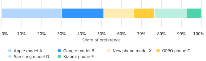
The primary focus in market simulations is on each product’s predicted market share based on participants’ predicted first choices – i.e. the products each participant is most likely to choose based on their utilities from the conjoint survey.
For example, as illustrated in Table 7 (from 1000minds’ market simulator), each phone’s predicted market share, or “share of preferences”, is calculated by dividing the number of participants for whom that product is their first choice by the total number of participants in the survey (e.g. 140 in the example below). The sum of market shares across all phones is 100% (1).
(This first-choice aggregation process is analogous to an election in which citizens vote for their preferred candidate with the votes tallied to calculate the vote shares or percentages.)
By observing how predicted market shares change under different pricing scenarios, the simulator models how sensitive demand is to price changes – exactly what price elasticity of demand is about.
| Name |
Market shares Participants’ 1st choice n=140 |
Attributes | |||||
|---|---|---|---|---|---|---|---|
| Operating performance |
Camera quality |
Battery life |
Screen quality |
Price | Size | ||
| Apple model A | 30% 42 |
very good | ok | very good (13+ hours) | very good | $1000 | large (6″) |
| Google model B | 21.1% 29.5 |
very good | good | good (11–12 hours) | very good | $900 | medium (5.5″) |
| New phone model X | 15% 21 |
good | very good | good (11–12 hours) | ok | $800 | large (6″) |
| OPPO phone C | 10.4% 14.5 |
good | good | ok (10 hours) | good | $600 | medium (5.5″) |
| Samsung model D | 16.4% 23 |
good | very good | very good (13+ hours) | very good | $1000 | small (5″) |
| Xiaomi phone E | 7.1% 10 |
ok | good | ok (10 hours) | good | $600 | large (6″) |
| Total | 100% 140 |
||||||
Pricing simulations
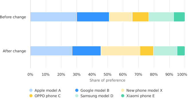
To run a pricing simulation in 1000minds, all you need to do is change the price of the product you’re considering and observe how its market share, or share of preferences, changes.
In the simulator, each product’s predicted market share is a proxy for quantity demanded, normalized by the number of participants in the simulated market (e.g. 140 in the example). The sum of market shares across all phones is 100% (1).
Own-price and cross-price elasticity coefficients
By comparing market shares before and after a price change, the simulator estimates both own-price and cross-price elasticity coefficients.
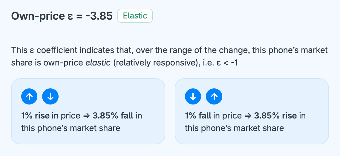
For example, as illustrated in Table 8, suppose the price of “New phone model X” is reduced by $100. Its predicted market share increases from 21% to 35.5%, producing an own-price elasticity coefficient of −3.85 (see Figure 1), where this coefficient was calculated using the arc method (explained in the technical note above).
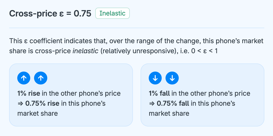
The cross-price elasticity coefficients associated with the $100 reduction in X’s price for the other five phones are also reported in Table 8 (see Figure 2 for “Apple model A”).
Cross-price elasticity coefficients associated with price decreases are generally positive (for substitutes) or zero (unrelated products).
These results arise because when a product’s price decreases, its market share typically rises, and therefore, because competing products are substitutes or unrelated products, their market shares will fall or remain unchanged.
Conversely, when a product’s price increases, its market share will usually fall, while competing products’ shares will usually rise or remain unchanged.
| Name |
Market shares Participants' 1st choice n=140 |
Price elasticities of demand ε (arc) |
Attributes | ||||||||
|---|---|---|---|---|---|---|---|---|---|---|---|
| Before | After | Change | Price | Operating performance | Camera quality | Battery life | Screen quality | Size | |||
| Apple model A | 30% 42 |
27.1% 38 |
-9.5% -4 |
0.75 | cross-price ε | $1000 | very good | ok | very good (13+ hours) | very good | large (6″) |
| Google model B | 21.1% 29.5 |
18.6% 26 |
-11.9% -3.5 |
0.95 | cross-price ε | $900 | very good | good | good (11–12 hours) | very good | medium (5.5″) |
| New phone model X | 15% 21 |
25.4% 35.5 |
+69% +14.5 |
-3.85 | own-price ε |
$800 → $700 |
good | very good | good (11–12 hours) | ok | large (6″) |
| OPPO phone C | 10.4% 14.5 |
8.6% 12 |
-17.2% -2.5 |
1.42 | cross-price ε | $600 | good | good | ok (10 hours) | good | medium (5.5″) |
| Samsung model D | 16.4% 23 |
15.4% 21.5 |
-6.5% -1.5 |
0.51 | cross-price ε | $1000 | good | very good | very good (13+ hours) | very good | small (5″) |
| Xiaomi phone E | 7.1% 10 |
5% 7 |
-30% -3 |
2.65 | cross-price ε | $600 | ok | good | ok (10 hours) | good | large (6″) |
| Total | 100% 140 |
100% 140 |
0% 0 |
||||||||
Demand curves
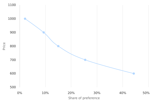
In addition to predicted market shares and price elasticities of demand, 1000minds’ market simulator can also generate demand curves for any products being analyzed (Figure 3).
What is a demand curve?
A demand curve is a simple graph showing the relationship between a product’s price and the quantity demanded by customers at different prices. It shows how customer demand responds across the range of possible prices.
1000minds’ market simulator generates demand curves by repeatedly changing the product’s price and calculating its predicted market share (or “share of preference”) at each price point. This predicted market share is a proxy for quantity demanded, normalized by the number of participants in the simulated market.
As illustrated in Figure 3 for “New phone model X”, demand curves slope downward: as price decreases, share of preferences increases; and vice versa: as price increases, share of preferences decreases. This is the same negative relationship captured by negative own-price elasticity coefficients discussed earlier.
This negative relationship between price and quantity demanded, or market share, is because, ceteris paribus (all else equal), when the price of something goes up, people demand less of it.
The “iron law” of demand
This negative relationship between price and quantity demanded is often described in Economics as the “iron law” of demand, reflecting how consistently it is observed. It can be explained in theoretical terms by two reinforcing effects:
- The substitution effect: As a product becomes more expensive, consumers switch to cheaper alternatives, and so buy less of the product
- The income effect: As the price rises, consumers’ purchasing power shrinks, meaning they can no longer afford to buy as much of the product
From simulating price changes to real-world testing
Market simulations are a powerful way to explore pricing decisions, but they are still just models of customer behavior rather than the behavior itself. The next step for a business is to validate and refine these insights in the real world while managing risk.
A sensible approach is to move from simulation to controlled experimentation. Rather than rolling out a new price across an entire market, a business can test it in a limited way, such as in specific regions, channels and customer segments.
A/B testing
A common method is “A/B testing”, in which two (or more) groups of consumers are shown different prices for the same product – e.g. one price/group is “A” and the other is “B” – and the two purchasing behaviors are compared.
This experimental approach allows businesses to directly observe how demand responds to price changes in practice and to assess whether the estimated own- and cross-price elasticities from the simulations hold up in reality.
Differences between predicted and actual outcomes can themselves be highly informative, pointing to factors such as competitor reactions, brand perceptions or other real-world influences not fully captured in the model.
It is also important to treat pricing as an iterative process. Insights from these real-world tests can then be fed back into updated models, improving future simulations and decisions.
Over time, this combination of conjoint-based market simulation and careful market testing helps build a more reliable understanding of demand, enabling businesses to price with greater confidence and flexibility.
Profit maximization!
Finally, although this article has focused on how pricing affects demand and revenue, it is important to recognize that the ultimate objective of most businesses is profit.
Pricing decision-makers therefore need to consider how changes in price affect both sales volume and margins, while also taking production, distribution and other costs into account.
In practice, this broader perspective means using elasticity insights not just to predict revenue outcomes, but to identify the price that maximizes profit – i.e. the difference between revenue and cost.
Test your knowledge
Answer this short multi-choice quiz to check your understanding of the ideas covered in this article.
Having understood price elasticity of demand and seen how conjoint analysis combined with market simulations can improve pricing decisions, the obvious next question is: which software should you use?
Why use 1000minds for conjoint analysis and market simulations?
1000minds is award-winning software for conjoint analysis, discrete choice experiments (DCEs) and multi-criteria decision analysis (MCDA). Used by businesses, governments, universities and researchers in more than 100 countries, it combines scientific rigor with ease of use.
At the core of 1000minds is its patented PAPRIKA method, an adaptive conjoint-analysis algorithm that asks simple pairwise-comparison questions and adjusts dynamically to participants’ responses. This approach minimizes respondent burden while producing high-quality preference data.
What sets 1000minds apart?
1000minds is designed to make sophisticated conjoint analysis accessible without sacrificing scientific validity.
Easy survey setup
Create and launch conjoint surveys quickly using an intuitive survey builder. Surveys can be customized with images, translated into any language, and distributed to large numbers of participants. The built-in AI Assistant can also suggest attributes and alternatives to help you get started quickly.
User-friendly participant experience
1000minds’ simple, conversational question format is easy for participants to understand and complete, helping improve engagement, completion rates and data quality.
Built-in analysis and market simulations
Results are generated automatically in real time, including utilities, market simulations, demand curves and price elasticity estimates. No manual statistical analysis is required.
Scientifically validated
1000minds is used at over 940 universities and research organizations worldwide and has been cited in 440+ peer-reviewed publications. 1000minds’ validity and reliability are widely recognized by researchers and practitioners alike.
Award-winning innovation
1000minds has received 18 software and innovation awards. The Consensus Software Award (sponsored by IBM and Microsoft) praised 1000minds for having “blended an innovative algorithm with a simple user interface to produce a tool of great power and sheer elegance.”
| 1000minds advantage | What it means | Why it matters |
|---|---|---|
| Adaptive conjoint analysis | Conjoint surveys (choice sets) adapt to each participant’s answers | Personalized and efficient, with no “design” issues |
| PAPRIKA method | Pairwise trade-offs in a simple, adaptive format | Low responder burden and high-quality data |
| Easy conjoint survey setup | Intuitive survey builder with customizable design | Launch studies quickly in any language or format |
| AI assistance | For suggesting attributes and alternatives | Get started quickly, and refine as you go |
| Automated real-time analysis | Built-in reporting and export tools | Results generated automatically |
| Market simulator | Turns conjoint survey results into predicted market outcomes | Explore “what-if” scenarios easily |
| Cluster analysis | Groups participants with similar preferences | Reveals market segments to inform targeting and design |
| High engagement | Simple, conversational question style | Higher response rates and reliable results |
| Scientific validity | Used at 940+ universities and research organizations | Trusted across academia, government and business |
| Award-winning innovation | Recognized by 18 software and innovation awards | Proven technology with real-world impact |
| Multi-criteria decision analysis (MCDA) | As well as conjoint analysis & DCE, 1000minds is used for MCDA | Ideal for decision-making and market research |
| Ready-to-go models | Large library of pre-built examples available | Ready-made templates for rapid setup |
Try 1000minds for free
Explore how 1000minds can support your work by creating a free account or book a demo with one of our friendly experts to learn more.
